- + The pilot: GPSS-Plus
GPSS-Plus: Discrete-Event and Continuous Systems Simulation Engine
GPSS-Plus is a discrete-event and continuous systems simulation engine aimed at modeling and analyzing the behavior of real systems over time. Its purpose is not to program applications, but to describe how a system works and observe its evolution under different conditions.
In essence, it operates as a digital laboratory where a set of entities (customers, products, vehicles, signals, or data packets) flows through a network of processes and resources with defined capacities and delays.
The goal is to transform a real-world system description into an executable model: from an industrial production line or a logistics chain, to data traffic in a network or an emergency protocol. By simulating thousands of scenarios in minutes, it enables forecasting, decision optimization, and the design of contingency protocols within a general-purpose simulation environment.
There are different approaches to system modeling, depending both on the interface and on the objective.
Discrete and/or continuous Drag & Drop based:
- DES: Built by connecting graphical blocks.
- Continuous modeling: Differential equation systems.
- Hybrid graphical + scripting: Combine DES with external code.
Discrete language-based approaches (domain-specific or general-purpose):
- With a proprietary DSL: Entirely textual languages such as classic GPSS.
- On top of general-purpose languages: Through simulation libraries.
Thanks to inheriting the core concepts of classic GPSS, GPSS-Plus sits in both worlds, using its own language to define the model instead of building on general-purpose languages, and reinforcing the role of textual description as the system representation over graphical diagrams.
The ultimate goal is that everything can be understood:
GENERATE 5
ADVANCE 10 {From:"Madrid", To:"Paris"}
TERMINATE
The main innovations introduced are:
1. Syntax: extended compatibility
The most significant change lies in how block and command parameters are handled. In classic GPSS, parameters A, B, C... offered a fixed and limited syntax.
Classic example:
ADVANCE 30,10 ; Wait between 30 and 40 time units
In GPSS-Plus, this structure is preserved but extended with a JSON-like format, allowing more details to be specified without breaking simplicity:
ADVANCE 30,10 {From:"Madrid", To:"Paris"}This makes it possible to integrate graphical, behavioral, or logical parameters without inventing new syntactic variants for each case.
2. Graphical visualization
GPSS-Plus visually represents entities and blocks using simple graphical elements: small “dots” moving across a canvas, following exactly the model flow. This representation allows observing the system in real time, immediately understanding its dynamics, and facilitating the detection of bottlenecks or unexpected behaviors during execution.
This visualization, absent in classic GPSS, introduces a new way of interacting with the model, where direct observation becomes a key validation and comprehension tool.
3. Virtual entities (VE)
Virtual entities help describe the invisible parts of the model. For those coming from other paradigms, they capture what was previously described externally in another language. For beginners, they are simply another type of entity.
In GPSS-Plus, everything that happens in the system unfolds over time and can be observed while it happens. To make this possible, all behaviors are treated the same way: as entities that move—abstract, visible, or even just a volume.
Virtual entities are not visualized, but they are complete entities that execute internal logic or system events. They exist to describe behavior using
ON_ENTER, aTIMER, orTIMEOUT, and they live within the model itself.Depending on their lifecycle, there are three main types:
- Reactors, which handle specific events and then disappear.
- Agents, which do not die and manage the model universe.
- Components, living entities that exist as part of another entity and die with it.
With this approach, the model becomes an ecosystem of concurrent executions. An entity can wait for a bus while answering a call; an agent can control traffic; the sun can rise and set without any main entity needing to handle it.
Many common concepts from procedural or object-oriented programming are reinterpreted: behavior is not encapsulated in hierarchical objects, but explicitly modeled as entities that coexist and act in parallel within the system.
There is no this, no parent, no child: everyone is a brother. Functions stop being one-off calls and become living procedures. There is no “this.breathe()” that always breathes the same way, but a person who walks and, at the same time, breathes different air.
4. Model auditing and V&V
By being described entirely as an explicit model, GPSS-Plus allows its behavior to be automatically analyzed, interpreted, and cross-checked. An artificial intelligence or external auditor can reconstruct what the system does, detect internal inconsistencies, and compare the modeler’s intent with the actual execution.
This capability introduces a natural evolution of classic verification and validation (V&V) processes, which no longer rely solely on manual review and statistical analysis. Coherence between history (H), model (M), and execution (E) is incorporated, laying the groundwork for a new validation approach.
5. Structured variables
In GPSS-Plus, variables (
SAVEVALUE,ASSIGN) can contain numbers, strings, arrays, or objects. This allows working with complex data structures directly in the model, without resorting to external languages or losing readability.ASSIGN DATA, {type:"Student", Name:"Antonio", Age:22, Grades:[8,5.8,6,8]}6. Hybrid discrete–continuous system
Continuous modeling in GPSS-Plus is based on a simple idea: dividing time into small frames. By executing these steps sequentially within the event queue, continuous behavior naturally emerges.
INTEGRATE,DYNAMIC,SOLVEare the basic tools that allow defining continuous system structures integrated into the same discrete core. RK4, Jacobian matrices, and Newton–Raphson make it possible to simulate fluids, voltages, or velocities using the same DSL.7. Sandbox, digital twins, and edge software
Simulation models can pursue three main objectives:
- Sandbox, focused on bounded simulation and result generation, with or without historical data preload.
- Digital twin, where the model accompanies a real system for verification, control, or predictive operation.
- Edge software, where the model itself is the system, running permanently as operational logic.
In the latter two cases, the model must interact with the external environment. GPSS-Plus enables this coupling through the BRIDGER, which acts as a generic bidirectional channel between the model and real physical systems.
From a language perspective, access to external resources is uniform: a database, a file, or a sensor are handled with the same syntax. Opening a relay or storing a data point is expressed with
BRIDGE_WRITE, and replacing aGENERATEthat simulates packet input with a subscription to a real motion sensor is almost immediate. The transition from sandbox to digital twin or edge software is therefore transparent.Thanks to Rehydration, the model not only connects to the real world but synchronizes with its ongoing state, allowing the simulator to “wake up” in the middle of a process without losing operational continuity after the last stored data, even after the model has been modified.
Other notable extensions:
In addition to these innovations, GPSS-Plus incorporates multiple extensions that enhance expressiveness, modularity, and power:
- New resources: new blocks such as
STOCK,RESTROOM,CONDITIONS, finite state machines that extend the classic palette (STORAGE,FACILITY...). - Dynamic resource creation: what would require manually dragging hundreds of blocks in Drag & Drop engines is achieved in GPSS-Plus with a simple
FOREACHloop and aNEWFACILITY. This is the key difference between a textual language and classic graphical interfaces. - Statistics: automatic collection of statistics for any resource or sequence, with graphical visualization.
- Behavior functions: automatic interpolations built from real or simulated data that encapsulate complex behaviors (e.g., different segments of a road or a machine).
- Native functions: tools such as
CONCAT,MERGE,PUSHextend the language without relying on external code. - Automatic charts: simply tabulating data generates charts within the simulation environment.
- Contexts (
CX$): each model can define independent contexts, ideal for creating reusable libraries, modules, or components. - Full debugging: the system allows detailed tracking of the event queue, each entity, resource, or variable, facilitating model analysis and correction.
- + Season 1: Hello World
- + A simple example
We will simulate a basic system where entities (customers) arrive at a resource (service counter), wait if it is busy, are served, and then leave. In this model:
- Arrivals: Customers arrive every 60 to 70 time units.
- Service: Service time at the counter ranges from 60 to 90 time units.
- Queues: If the counter is busy, customers wait.
- Departure: Customers take 10 time units to move into the queue and another 10 to leave after service.
For those familiar with classic GPSS, we would have:
GENERATE 60,10   ; Entities are generated every 60 to 70 time units.
ADVANCE 10       ; Takes 10 time units to move into the counter queue.
SEIZE VENTANILLA ; The entity arrives at the counter queue.
ADVANCE 60,30    ; Service time: 60 to 90 time units.
RELEASE VENTANILLA ; Leaves the counter.
ADVANCE 10       ; Takes 10 time units to leave.
TERMINATE 1      ; The entity finishes.
START 100        ; Executes until 100 entities have been served.
In GPSS-Plus, it is very similar, but with graphical representation. To achieve this, we configure resources and additional parameters:
FACILITY {NAME:VENTANILLA, X:300, Y:300} ; Define the counter in space.
POSITION {NAME:SALIDA, X:500, Y:300}    ; Define the exit in space.

GENERATE 60,10 {NAME:GEN1, X:100, Y:300} ; Position the entity generator.
ADVANCE 10 {TO:VENTANILLA}               ; Move towards the counter.
SEIZE VENTANILLA                        ; Assignment of the "VENTANILLA" resource.
ADVANCE 60,30                           ; Service time: 60 to 90 time units.
RELEASE VENTANILLA                      ; Release of the resource.
ADVANCE 10 {TO:SALIDA}                  ; Move towards the exit.
TERMINATE 1                             ; The entity finishes.
START 100                               ; Executes until 100 entities have been served.
Final step: Press Play and observe the result. The first entity will exit the "Generate" block between time 60 and 70.
As can be observed, the program has not changed much to add the graphical component. Basically, we have defined the spatial layout of the elements.
- + Syntax: Commands and blocks
In a simulation, there are two main elements at play:
1. ENTITIES, or transactions, are the elements that change their state during the simulation. They can represent people, boxes, or any kind of item. In GPSS-Plus, they are represented as colored dots. These entities interact with the environment. For example, they enter the system through the
GENERATEblock, move through a circuit usingADVANCE, and terminate at aTERMINATEblock.2. RESOURCES, which make up the environment and are used by entities, such as a service counter or a container larger than the entity itself.
For example, a person (entity) approaches a service counter (resource). This counter is defined by a COMMAND, and a set of BLOCKS describe what the person does in relation to that counter.
An example of defining a resource as a service counter is the COMMAND:
FACILITY {name:Ventanilla1, x:100, y:100}An example of an instruction for an entity to occupy that counter is the BLOCK:
SEIZE Ventanilla1
In summary, the language is based on two main elements: blocks and commands.
1. Blocks bound to entities
Blocks are instructions that ENTITIES execute directly during the simulation. Each block defines a specific action that affects the flow or state of that entity.
General syntax:
BLOCK [PARAMETERS A,B,C..] {JSON-LIKE OPTIONS}
Block examples:
ASSIGN variableName,10
TERMINATE 1
Parameters are named by letters (A, B, C, ...). Depending on the block, they may also include parameters in a JSON-like format, usually defining graphical or advanced aspects.
Example:
MOD {COLOR:#FF0000} ; sets an entity to red color.Another example:
ADVANCE 10,5 {TO:Ventanilla1} ; the entity advances in time towards "Ventanilla1"2. Commands bound to resources and the engine environment
Commands configure the simulation environment. Unlike blocks, they are not executed directly by entities. Instead, they define resources, graphical positions, and system rules.
General syntax:
COMMAND {NAME:theName, JSON-LIKE OPTIONS}
Example of defining a storage resource:
STORAGE {NAME:ALMACEN1, CAPACITY:10, X:270, Y:200}This format allows adding additional information such as position (X, Y).
- + Variables: Savevalues and Assigns
In GPSS-Plus, variables allow storing information that can be used by entities or to configure elements of the environment. These variables are mainly divided into two types:
1. SAVEVALUE (global variables): Global variables are accessible by any entity and persist throughout the entire simulation. They are useful for storing shared data such as counters, accumulators, or global states.
Syntax:
SAVEVALUE variable, valueExample:
SAVEVALUE TiempoEspera, 8
This command sets the global variable "TiempoEspera" to a value of 8.
Once defined, the value can be updated at any time:
SAVEVALUE TiempoEspera, 10
The value of "TiempoEspera" is now 10.
To retrieve the value of a global variable, SNA are used, which follow a specific format:
X$savevalueName or X$(savevalueName)
; X$TiempoEspera or X$(TiempoEspera)

IF (X$TiempoEspera > 10)
...
For example, incrementing the value of a savevalue can be done as follows:
SAVEVALUE TiempoEspera, X$TiempoEspera + 1
Or through the method:
SAVEVALUE.inc TiempoEspera
In particular, since these variables are used by more than one entity, they have an associated COMMAND for creation and initialization called
INITIAL.Its syntax is simple:
INITIAL TiempoEspera,10
Remember that
INITIALis a command. It is used at the beginning of the program for initialization.2. ASSIGN (entity local variables):
Local variables belong to a specific entity. Each entity can have its own value for the same variable, which makes them useful for managing entity-specific data.Syntax:
ASSIGN variable, valueExample:
ASSIGN Identificador, 1
This block assigns the value 1 to the variable "Identificador" of the current entity invoking ASSIGN.
To retrieve the value of a local variable using its SNA format:
P$assignName or P$(assignName)
; P$Identificador or P$(Identificador)
if (P$Identificador > 5) ...
P$Identificador is the form that allows obtaining the value of a local variable of the entity.
Key differences between SAVEVALUE and ASSIGN:
- Scope: SAVEVALUE variables are global, while ASSIGN variables are entity-local.
- Persistence: SAVEVALUE variables retain their value at all times, even if no entity uses them. ASSIGN variables only exist while the entity is active.
- Usage: Use SAVEVALUE for shared data, and ASSIGN for entity-specific data.
Combined example:
In this example, we combine SAVEVALUE and ASSIGN to calculate the average waiting time at a service counter. If the time is defined by an ADVANCE 15,10, it means it will range between 15 and 25 time units. This should gradually approximate the average to 20.
INITIAL TiempoTotal, 0
INITIAL NumEntidades, 0
Facility {NAME:Ventanilla,X:354,Y:204}
Graphic {NAME:Text1,Type:TEXT,X:358,Y:321,Text:"Average"}
Position {NAME:Salida,X:577,Y:201}
START 50
;---------------------------------

Generate 20,0 {NAME:GEN1,X:100,Y:207}
ADVANCE 10 {to:Ventanilla}
SEIZE Ventanilla
ASSIGN TiempoInicio, AC1$
ADVANCE 15,10
ASSIGN TiempoFinal, AC1$
RELEASE Ventanilla
ADVANCE 15 {to:Salida}
ASSIGN TiempoEntidad, (P$TiempoFinal - P$TiempoInicio)
SAVEVALUE NumEntidades, X$NumEntidades + 1
SAVEVALUE TiempoTotal, X$TiempoTotal + P$TiempoEntidad
SAVEVALUE promedio, round(X$TiempoTotal / X$NumEntidades,3)
MOVE {NAME:Text1,text:"Average: X$promedio"}
TERMINATE 1
In this code:
- Each entity calculates its waiting time at the service counter.
- Times are accumulated in the global variable "TiempoTotal".
- The number of served entities is counted in "NumEntidades".
- At the end of the simulation, you can compute the average waiting time:
AverageTime = X$TiempoTotal / X$NumEntidadesIn this way,
SAVEVALUEandASSIGNwork together to provide efficient data handling within the simulation.Later on, we will see how both BLOCKS support much more than just numerical variables.
- + Structure: IF, CALL, PROCEDURE
In this example, we simulate a system where each entity randomly chooses one of three service counters to be served. Each counter has its own queue, and the flow is unevenly distributed depending on the service time.
The decision logic is resolved exclusively through structured procedures.
FACILITY {NAME:VENTANILLA1,X:320,Y:450}
FACILITY {NAME:VENTANILLA2,X:320,Y:300}
FACILITY {NAME:VENTANILLA3,X:320,Y:150}

POSITION {NAME:POS1,X:160,Y:300}
POSITION {NAME:POS2,X:497,Y:300}

START 30 ; Executes until 30 entities are completed

GENERATE 10,0 {NAME:GEN1,X:60,Y:300}
ADVANCE 20,0 {TO:POS1}
ASSIGN ALEATORIO,RANDOM
IF (P$ALEATORIO < 0.3)
    CALL CAMINO1
    ELSE
       IF (P$ALEATORIO < 0.6)
          CALL CAMINO2
          ELSE
          CALL CAMINO3
       ENDIF
ENDIF
ADVANCE 20 {TO:POS2}
TERMINATE 1

;---------------------------------------------

PROCEDURE CAMINO1
ADVANCE 20  {TO:VENTANILLA1}
SEIZE VENTANILLA1
ADVANCE 25,10
RELEASE VENTANILLA1
ENDPROCEDURE

PROCEDURE CAMINO2
ADVANCE 20 {TO:VENTANILLA2}
SEIZE VENTANILLA2
ADVANCE 10,2
RELEASE VENTANILLA2
ENDPROCEDURE

PROCEDURE CAMINO3
ADVANCE 20 {TO:VENTANILLA3}
SEIZE VENTANILLA3
ADVANCE 10,2
RELEASE VENTANILLA3
ENDPROCEDURE
Compared to the previous example, only a few new BLOCKS are introduced:
ASSIGN ALEATORIO,RANDOM
This block creates a local variable in the entity (called
ALEATORIO) and assigns it a random number between 0 and 1, using theRANDOMfunction.These local variables are also called parameters and are accessed using the SNA notation:
P$ALEATORIO- "P" because it is a parameter,
- "$" is the standard separator,
- "ALEATORIO" is its name.
IF (P$ALEATORIO < 0.3)
This is an "IF" control-structure block.
As can be seen, it is an "if" just like in any other language: a variable is compared against a value.
This other control-structure block also needs little introduction. It calls a PROCEDURE:
CALL CAMINO1
Finally:
PROCEDURE CAMINO1
...
ENDPROCEDURE 100 ; would produce an ASSIGN in the calling entity named CAMINO1 with value 100
Which also requires little explanation. PROCEDURE blocks encapsulate a set of actions.
ENDPROCEDUREmay include a value in parameter A, which is returned in the same way as if anASSIGNinstruction had been generated. It can be retrieved as P$ProcedureName (e.g., P$CAMINO1). In this case, it is not used. - + Resources: Storage
One of the classic resources is
STORAGE.FACILITYrepresents things such as a service counter, a machine, or an operator: it can serve only one entity at a time and according to its capacity (with CAPACITY:3, the FACILITY would serve 3 entities). STORAGE, on the other hand, represents something like a warehouse, a tank, or a network that can be used partially.What is a
STORAGE? ASTORAGEis a type of resource that is not seized per entity, but by quantity. It is used when an entity must reserve part of a resource without occupying it entirely. For example, a truck can drop 10 boxes into a warehouse that can hold up to 40.How does it work? It is defined with a total capacity, for example 40 units.
STORAGE {NAME:warehouse1, X:300, Y:200, capacity:40}Entities use the
ENTERblock to occupy a certain amount, andLEAVEto give it back.ENTER warehouse1,5 LEAVE warehouse1
If an entity tries to occupy more than what is available, it will automatically wait in an internal queue until the
STORAGEhas enough free capacity. You don’t need to program anything additional to manage that wait.In the example: a box warehouse (
STORAGE) is defined with 40 capacity units. Trucks arrive every 10 time units and deposit between 1 and 16 boxes. After some time, they leave, freeing the occupied space. You will see on-screen text how many boxes are stored at any moment.In addition to calculating it via additions and subtractions, you can also do it directly by querying the corresponding SNA for
STORAGEoccupancy:R$(warehouse1,OCCUPIED) ; Units currently occupied R$(warehouse1,LEFT) ; Units available
Example:
/* Warehouses: STORAGE Capacity management and storage usage. */ INITIAL capacity,40 ; defines a savevalue named capacity with value 40 STORAGE {NAME:warehouse1, X:300, Y:200, capacity:X$capacity} POSITION {NAME:EXIT, X:500, Y:200} ; Text showing current contents GRAPHIC {NAME:text1, Type:TEXT, X:320, Y:240, Text:"Current boxes: 0"} START 100 ; Trucks arriving every 10 time units GENERATE 10,0 {NAME:Truck, X:100, Y:200} ADVANCE 15 {TO:warehouse1} ENTER warehouse1,(random*15)+1 ; Occupies between 1 and 16 storage units savevalue usage,X$capacity - R$(warehouse1,LEFT) MOVE {name:text1,text:"Current boxes X$usage : R$(warehouse1,OCCUPIED)"} ADVANCE 40,10 LEAVE warehouse1 ; Releases the occupied units savevalue usage,X$capacity - R$(warehouse1,LEFT) MOVE {name:text1,text:"Current boxes X$usage : R$(warehouse1,OCCUPIED)"} ADVANCE 15 {TO:EXIT} TERMINATE 1 - + The event queue: the simulation engine
The event queue:
At the heart of any discrete-event simulation lies the event queue, a structure that defines how and when entity actions are executed within the model. This discrete-event approach is what distinguishes it from other programming languages.
You can think of it as if each entity had its own program, as you would do in C or Python, but jumping between entities according to the temporal order dictated by this queue. If we simulate 10 entities, there are 10 programs running “at the same time” (or almost).
What is the event queue?
It is a time-ordered list of scheduled actions, each associated with a simulated time instant (AC1). The queue ensures actions are executed in the correct order according to when they must occur.
The most important thing: it is ordered by time. For example:
Time 15 - Serve entity 14 at step 88
Time 45 - Serve entity 22 at step 16
Time 77 - Serve entity 16 at step 25
Example: Evolution of the event queue
Let’s consider the classic case of a bank where customers enter through the door and are served at a counter. Entities are created with
GENERATEand spend time being served viaADVANCE.Imagine we are at instant
T = 5, with the following queue:T 5: Entity 5: Waiting in the counter queue T 7: GENERATE: Create an item, a customer who will enter through the door T 8: Entity 9: Heading to the counter queue T 16: Entity 3: Heading to the counter queue
Right now, we have one entity—#5—which is next in the queue. We will remove that element from the queue to process it. Now we know that time is 5! Not because time has “passed”, but because our next task is scheduled for T=5.
Let’s assume, for example, that Entity 5 is at the “step” (position in its program) that indicates an
ADVANCE 10to be served.In that case, the solution is to schedule itself in the queue at T=15 (5+10) and pause its execution while it is being served.
Now the event queue will look like this:
T 7: GENERATE: Create an item
T 8: Entity 9: Heading to the counter queue
T 15: Entity 5: Go to the exit
T 16: Entity 3: Heading to the counter queue
We are now at the next event. Time must be updated again: “AC1” now takes the value 7. As we said, it’s not that time has passed; it’s that the event queue makes time jump because there is nothing to do until T=7.
We remove the element from the queue and find a
GENERATE 20,5. Therefore, we must compute what time is defined by 20,5; something between 20 and 25. Suppose the result is 22. That is, another person will enter in 22 time units. The queue now takes this form after theGENERATEadvances and performs 2 tasks:1.- The
GENERATEitself advances 20 (parameter A) (7+20=27).
2.- It creates a new entity (#10) so it can carry out its tasks 22 time units later (7+22=29).T 8: Entity 9: Heading to the counter queue T 15: Entity 5: Go to the exit T 16: Entity 3: Heading to the counter queue T 27: GENERATE: Create an item T 29: Entity 10: Heading to the counter queue
Now it would be time to advance system time again and serve the next element: Entity 9.
This event queue will remain alive until one of the program-ending conditions is met.
In GPSS-Plus, this event queue also has additional characteristics to support tasks in the graphical world and to add “ON_*” type events.
In the GPSS-Plus event queue, we have 5 types of elements:
- GENERATE – Introduce new entities into the system.
- Entities – The ones that move through the model and consume resources.
- Dead times – Visible pauses that allow step-by-step simulation or speed adjustment.
- Virtual entities – Not visible; execute events such as ON_ENTER, ON_TIMER, etc.
- System TIMER – Like a GENERATE, but it produces virtual entities at fixed intervals.
Resource queues:
Other existing queues are those belonging to resources; each resource can have one or two depending on the case.
These lists are ordered by arrival order, and their management depends exclusively on the resource itself.
For example, a
FACILITYhas two lists: the list of occupying entities and the list of entities waiting in queue.When an entity attempts to
SEIZE, if the resource is busy, it moves to the waiting list. If there are no entities in the resource, it will seize it by entering the occupants list.When it performs
RELEASE, it leaves that list and forces the resource to look for an entity in its pending queue to enter. If there is one, it will move it into the occupants list and schedule its entry into the event queue at that same instant, so that entity will take control of the engine as soon as the departing one stops its activity.Conclusion
The event queue not only defines the order and time at which actions occur, but also acts as the core of the system. It ensures blocks execute correctly and that the simulation is consistent and accurate. Understanding this concept is essential to design efficient models and fully leverage GPSS-Plus capabilities.
In GPSS-Plus it is easy to view this queue: just open the menu window and click the “Event Queue” button.
- + Conditions: Waiting for a condition
Imagine a group of people waiting for an automatic door to open. They are not queuing and they are not occupying anything; they are simply waiting for something to happen.
This is exactly what the
CONDITIONSresource allows: stopping entities until a logical condition is met.Something similar existed in classic GPSS with the
ASSEMBLEblock for this purpose. In GPSS-Plus, this behavior is replaced by a more general and flexible resource.The
CONDITIONSresource allows holding entities until a condition is satisfied. This condition is defined as an expression that is evaluated each time an entity attempts to pass.CONDITIONS {NAME:Conditions1,X:208,Y:317,expression:(X$counter>=5)}CONDITIONShas additional options that will be covered later.Its associated block,
WAITUNTIL, is responsible for validating the condition for the current entity — in this case, whether the counter is greater than or equal to 5.When the 5th entity arrives, the condition is satisfied and it continues without being held. At that point, the remaining entities are released by checking all retained ones using another associated block:
WAITCHECK.It is interesting to observe that all entities leave the
CONDITIONSresource together in the first segment. In the second one, the randomness ofADVANCE 20,40causes them to spread apart.We also begin using the
ENDGENERATEblock, which is more consistent with the structured approach thanTERMINATE. They are equivalent, but syntactically it is more appropriate to structure the block usingGENERATE/ENDGENERATE. This makes it easier to identify which block was generated, especially when multipleGENERATEblocks exist in the program.
Example:
/* Synchronization: CONDITIONS / WAITUNTIL Entities wait as a group and advance together. */ POSITION {NAME:POS1,X:208,Y:222} POSITION {NAME:POS2,X:452,Y:215} POSITION {NAME:POS3,X:752,Y:215} CONDITIONS {NAME:Conditions1,X:208,Y:317,expression:(X$counter>=5)} ; Holding resource INITIAL counter,0 START 100 ;***************************************************** GENERATE 10,2 {NAME:GEN1,X:86,Y:228,ERADIO:10,ECOLOR:#FF9900} ADVANCE 16,0 {TO:POS1} SAVEVALUE counter, X$counter + 1 WAITUNTIL Conditions1 WAITCHECK Conditions1 SAVEVALUE counter, 0 ADVANCE 20,0 {TO:POS2} ; ALL entities advance together to the second position ADVANCE 20,40 {TO:POS3} ; Advance to the third position with random time between 20 and 40, now SPLITTING ENDGENERATE 1 ; Ends the life of the entity — IDENTICAL to TERMINATE 1 - + Second structural step
Now that you already know how to use procedures and simple conditional decisions (
IF), let’s look at a case where an entity chooses between multiple possible routes.For this, we use the
SWITCHstructure, very similar to a “decision menu”.What does this example do?
- Generates an entity every 10 time units.
- Assigns it a random number (
P$RANDOM_VALUE). - Depending on that number, chooses one of four routes (
CALL PATH1…CALL PATH4). - In two of those routes (PATH3 and PATH4), a visual block is activated showing “Lock” or “Unlock”, and resources are locked or unlocked. If an entity enters path 3, the use of resources 1, 2, and 3 is locked, although entities already inside them are allowed to finish their work. When an entity takes path 4, those resources become available again immediately. Locking does not expel entities already using the resources, but prevents new ones from seizing them until they are unlocked.
We also define a purely visual aspect: “flow”.
By enabling it inADVANCE, we will see a route line that initially runs vertically or horizontally depending on theLAYOUT. It may pass through aVIAorVIA2, and can converge or diverge according toMERGEorDECISION.
Example:
/* Blocks: SWITCH and LOCK/UNLOCK Conditional routing and management of lockable resources. */ FACILITY {NAME:COUNTER1,X:320,Y:450,CAPACITY:3} FACILITY {NAME:COUNTER2,X:320,Y:300,CAPACITY:3} FACILITY {NAME:COUNTER3,X:320,Y:150} FACILITY {NAME:COUNTER4,X:320,Y:50} POSITION {NAME:POS1,X:158,Y:301} POSITION {NAME:POS2,X:497,Y:300} POSITION {NAME:POS3,X:627,Y:300,TYPE:TERMINATE,TITLE:END} GRAPHIC {NAME:Text1,Type:TEXT,X:320,Y:104,Text:"Unlock"} START 30 GENERATE 10,0 {NAME:GEN1,X:57,Y:300} ADVANCE 20,0 {TO:POS1,flow:1} ASSIGN RANDOM_VALUE,(RANDOM) SWITCH P$RANDOM_VALUE CASE <,0.4 CALL PATH1 ENDCASE CASE <,0.8 CALL PATH2 ENDCASE CASE <,0.92 CALL PATH3 MOVE {NAME:Text1,text:"Lock"} LOCK COUNTER1 LOCK COUNTER2 LOCK COUNTER3 ENDCASE DEFAULT CALL PATH4 MOVE {NAME:Text1,text:"Unlock"} UNLOCK COUNTER1 UNLOCK COUNTER2 UNLOCK COUNTER3 ENDCASE ENDSWITCH ADVANCE 20,10 {TO:POS2,flow:1,MERGE:"exit"} ADVANCE 20,0 {TO:POS3,flow:1} ENDGENERATE 1 ;**************************************** PROCEDURE PATH1 ADVANCE 20 {TO:COUNTER1,flow:1,DECISION:"start"} SEIZE COUNTER1 ADVANCE 45,10 RELEASE COUNTER1 ENDPROCEDURE PROCEDURE PATH2 ADVANCE 20 {TO:COUNTER2,flow:1,DECISION:"start"} SEIZE COUNTER2 ADVANCE 40,10 RELEASE COUNTER2 ENDPROCEDURE PROCEDURE PATH3 ADVANCE 20 {TO:COUNTER3,flow:1,DECISION:"start"} SEIZE COUNTER3 ADVANCE 40,20 RELEASE COUNTER3 ENDPROCEDURE PROCEDURE PATH4 ADVANCE 20 {TO:COUNTER4,flow:1,DECISION:"start"} SEIZE COUNTER4 ADVANCE 10,2 RELEASE COUNTER4 ENDPROCEDURE ;*************************************************************** - + A complete model
Now that you know the fundamentals of GPSS-Plus, let’s see how they all come together in a unified example.
We’re going to look at a piece of code that is quite a bit longer than what we’ve seen so far—almost 100 lines.
This model represents a system with different vehicle types that move through a work area for several cycles. Each one decides its route, performs tasks, and finishes after completing a number of cycles, entering the utility-vehicle or truck parking area as appropriate—occupying either a
FACILITYor aSTORAGEdepending on the truck size.This code introduces several new ideas.
The first thing we notice is a top-level structure with two
GENERATEblocks and severalPROCEDUREs.The generates are visually separated so each one has its own activity, and they mark the entities born from them in a differentiated way.
GENERATE ... NAME:G_UTILITY_VEHICLES ; generates utility vehicles
   ....
   ASSIGN ...
   ....
   CALL PROC.MAIN
ENDGENERATE 1
And then we have the set of
PROCEDUREs:Process procedures:
PROC.MAIN              ; Main process
PROC.UTILITY_VEHICLES
PROC.TRUCKS
Decision procedures:
DECIDE.ROUTE
DECIDE.LOOP_OR_END
PROC.MAIN:
All the main logic is concentrated in the PROC.MAIN process, which is typically built around a
WHILEloop that keeps entities inside until they meet the condition to finish all their tasks.WHILE ("P$state"!="EXIT") ... ... ASSIGN state, ???? ENDWHILEInside it, the decision over the main routes each entity can take is typically a
SWITCHwith options or several nestedIFs. It is a good practice to place these decisions intoPROCEDUREs namedDECIDE.*, so they are easy to recognize and you know in advance they usually return, directly, the name of thePROCEDUREto be invoked by the entity:ENDPROCEDURE "P$VALUE" ; Will return 'PROC.UTILITY_VEHICLES' or 'PROC.TRUCKS'
That is: CALL DECIDE.AAA will return in P$AAA (the part before the dot is omitted) the value 'PROC.BBB', which can be used directly as CALL P$AAA.
CALL DECIDE.ROUTE           ; Executes decision logic
CALL "P$(ROUTE)"            ; Calls the procedure returned by the decision
Very similar to the decision to exit or continue looping through the cycle.
Other new elements are:
ADVANCE0 {TO:POS_ENTRY,flow:1,layout:H}Here it is
ADVANCE0instead ofADVANCEbecause we only want a visual jump, without the entity consuming time by entering and leaving the event queue.The last novelty is the use of another resource with grouping and statistics utility:
QUEUER.It has unlimited capacity and makes it easy to know how many—and which—entities are in a given zone.
QUEUE IN_PARKING  ; enter
...
...
DEPART IN_PARKING ; leave
In summary, the example shows:
- How to use multiple
GENERATEblocks with differentiated logic (trucks and utility vehicles). - How entities can dynamically decide routes (
SWITCH,CALL,PROCEDURE). - How an internal per-entity loop (
WHILE) is used to simulate iteration. - How to visualize flow using positions, subtitles, and styles.
- How to combine different resources (
FACILITY,STORAGE,QUEUE). - How to work with dynamic procedure names (
P$(ROUTE)).
Example:
QUEUER {NAME:IN_PARKING,X:413,Y:497} FACILITY {NAME:UTILITY_VEHICLES, CAPACITY:4, X:413, Y:390} STORAGE {NAME:TRUCKS, CAPACITY:5, X:412, Y:120} POSITION {NAME:POS_ENTRY,X:240,Y:270} POSITION {NAME:POS_EXIT,X:557,Y:316,TYPE:DECISION,TITLE:"END?"} POSITION {NAME:POS_LOOP,X:225,Y:549} POSITION {NAME:END,X:730,Y:324,TYPE:TERMINATE} START 20 ;************************************************************************ GENERATE 20,10,0,10 {NAME:G_UTILITY_VEHICLES,X:80,Y:363,ESUBTITLE:"P$cycles/3"} ASSIGN VEHICLE_TYPE,1 MOD {RADIO:5,COLOR:#000066} CALL PROC.MAIN ENDGENERATE 1 ; ALIAS OF TERMINATE ;---------------------------- GENERATE 20,10,0,10 {NAME:G_TRUCKS,X:80,Y:199,ESUBTITLE:"P$cycles/3"} ASSIGN VEHICLE_TYPE,FLOOR(RANDOM * 2 + 2) MOD {RADIO:10,COLOR:#006600} CALL PROC.MAIN ENDGENERATE 1 ; ALIAS OF TERMINATE ;************************************************************************ PROCEDURE PROC.MAIN ASSIGN cycles,1 ADVANCE0 {TO:POS_ENTRY,flow:1,layout:H} ASSIGN state,"loop" WHILE ("P$state"!="EXIT") QUEUE IN_PARKING CALL DECIDE.ROUTE ; return assign:ROUTE CALL "P$(ROUTE)" ADVANCE 20,18 {TO:POS_EXIT,flow:1,MERGE:"exit"} DEPART IN_PARKING CALL DECIDE.LOOP_OR_END ASSIGN state,"P$(LOOP_OR_END)" ENDWHILE ADVANCE 20,0 {TO:END,flow:1} ENDPROCEDURE ;***************************************************** PROCEDURE DECIDE.ROUTE ASSIGN VALUE,"" SWITCH P$VEHICLE_TYPE CASE <=,1 ASSIGN VALUE,"PROC.UTILITY_VEHICLES" ENDCASE DEFAULT ASSIGN VALUE,"PROC.TRUCKS" ENDCASE ENDSWITCH ENDPROCEDURE "P$VALUE" ;--------------------------------------------- PROCEDURE DECIDE.LOOP_OR_END ASSIGN VALUE,"loop" ASSIGN cycles,P$cycles + 1 IF (P$cycles > 3) ASSIGN VALUE,"EXIT" MOD {SUBTITLE:"-EXIT-"} ELSE ADVANCE 30 {TO:POS_ENTRY,flow:1,VIA:POS_LOOP,layout:V} ENDIF ENDPROCEDURE "P$VALUE" ;--------------------------------------------- PROCEDURE PROC.UTILITY_VEHICLES ADVANCE 20 {TO:UTILITY_VEHICLES,flow:1,DECISION:"resource"} SEIZE UTILITY_VEHICLES ADVANCE 55,40 RELEASE UTILITY_VEHICLES ENDPROCEDURE PROCEDURE PROC.TRUCKS ADVANCE 20 {TO:TRUCKS,flow:1,DECISION:"resource"} ENTER TRUCKS, P$VEHICLE_TYPE ADVANCE 40,20 LEAVE TRUCKS ENDPROCEDURE ;---------------------------------- - How to use multiple
- + A simple example
- + Season 2: Virtual Entities (VE)
- + Entities and virtual entities (VE)
By now we have more than enough clarity on what an entity is: a little dot moving on the screen. We know it is born from a
GENERATE, it traverses blocks, advances through positions, and can enter resources.So what is a virtual entity? An entity that does not move on the screen.
That difference sounds simple, but it is essentially that—while carrying many implications. Imagine an invisible dot that does not occupy space but still executes instructions.
Let’s define them formally:
- Virtual entities are not born from a
GENERATE. Instead, they are created by COMMANDS such asTIMER,PRE_RUN,TRIGGER(ON_ENTER,ON_QUEUE,ON_*...), or by the blockTIMEOUT. - Their identifier (D$N) is not a positive sequential number (1, 2, ... n) but the opposite: (-1, -2, ... -n).
- Their
TERMINATEdoes not subtract terminations. In fact, you will seeTERMINATE_VE, which ends only virtual entities. - They have no direct visual representation, but they can interact with the graphical layer just like any other entity.
What are they for?
They have countless uses.
Even if it may not look like it, they are the reason GPSS-Plus does not rely on secondary languages to program complementary elements such as Python or Java.
You program them in GPSS-Plus like any other subprogram. They take care of all accessory tasks around entity life cycles. For example, if you want a clock, it makes little sense for it to depend on the birth or movement of entities that already have plenty to worry about while entering and leaving resources.
Instead, aTIMERthat automatically fires every N instants can do those tasks.
If you want control over multiple resources and the state of their queues, you can have a virtual entity acting as a controller each time an entity enters a queue.Virtual entities work behind the scenes. You don’t see them move, but without them, many processes simply would not happen.
In the example:
A normal entity, number 1 (
D$N==1), creates a virtual entity that will be born in 30 time units to execute a procedure:TIMEOUT updateCounter,30
It does not traverse flow positions nor use resources. It only appears after being requested by an entity and, from then on, the virtual entity schedules a new virtual entity every 3 time units.
Its only job: counting.
The first calls the second, which calls the third... all through theTIMEOUTblock, which only needs the name of the procedure to be executed by the virtual entity and the time at which it will occur.
You can see the text changing even though there are no visible entities updating it. That is because a virtual entity does it, working in the background like a small autonomous process.This example shows how a VE can act as a recurring process without any human intervention or physical entity. From now on, you will see that many system decisions, alarms, or statistics will be managed by this type of invisible entity.
Example:
/* Virtual entities: Invisible processes operating in the background. The first entity will create a VE after a delay of 30 time units. That VE will create the next one every 3 time units. Only entities are visible, not VEs. */ POSITION {NAME:POS1,X:321,Y:332} POSITION {NAME:POS2,X:517,Y:326} GRAPHIC {NAME:Text1,Type:TEXT,X:366,Y:454,Text:"Counter: 0"} INITIAL counter,0 START 200 ;***************************************************** GENERATE 20,0 {NAME:GEN1,X:101,Y:332} ADVANCE 10 {TO:POS1} ; Launch a virtual entity that will update the counter IF (D$N==1) TIMEOUT updateCounter,30 ENDIF ADVANCE 10 {TO:POS2} ENDGENERATE 1 ;***************************************************** PROCEDURE updateCounter SAVEVALUE counter, X$counter + 1 MOVE {NAME:Text1, TEXT:"I am Virtual Entity D$N. Counter: X$counter"} TIMEOUT updateCounter, 3 TERMINATE_VE ENDPROCEDURE - Virtual entities are not born from a
- + Creation of virtual entities (VE)
We have already seen what a virtual entity is: an entity that does not move on the screen but still executes instructions and participates in the simulation engine.
Now we will see how these virtual entities are created and who can create them.
Who creates a VE?
Virtual entities are not born from a
GENERATEblock like normal entities. Instead, they can be created by four different mechanisms:- The system, using:
PRE_RUN– at the beginning of the simulation, once.TIMER– at fixed intervals defined byINTERVAL.
- An entity, using:
TIMEOUT– schedules the execution of a VE X time units in the future.
- A resource, using
ON_*events such as:ON_SEIZE,ON_RELEASE,ON_LEAVE, etc.
What do they all have in common?
All virtual entities execute a
PROCEDURE, which may be specified as aTRIGGERor as a procedure name. ThatPROCEDUREis the “code” executed by the VE. It must end withTERMINATEorTERMINATE_VE, just like any normal entity.About parameters
When using
NEW,TIMEOUT, orCALL, we can pass additional parameters. These will be available inside the procedure asP$PARAM_A,P$PARAM_B, etc., just as we have already seen withCALL.This allows a VE to “know” who invoked it or why.
In the example:
PRE_RUNcreates an entity at the start (magenta color).TIMER1creates one every 53 time units (blue color).TIMEOUTfires just before entering the resource and leaves a message.ON_RELEASEfires whenFACILITY1is released.
Each time one of these virtual entities is created, a message appears on screen showing its identifier and what it is doing.
Example:
/* Creation of virtual entities */ SYSTEM {TYPE:ON_TIMER, TRIGGER:TIMER1, INTERVAL:53} SYSTEM {TYPE:PRE_RUN, TRIGGER:PRE_RUN} POSITION {NAME:POS1,X:311,Y:497} POSITION {NAME:POS2,X:571,Y:147,TYPE:TERMINATE,TITLE:END} FACILITY {NAME:Facility1,X:573,Y:483,ON_RELEASE:on_RELEASE_Facility1} GRAPHIC {NAME:Text_Pre_run,Type:TEXT,X:253,Y:196} GRAPHIC {NAME:Text_TIMER1,Type:TEXT,X:253,Y:158} GRAPHIC {NAME:Text_Timeout1,Type:TEXT,X:254,Y:252} GRAPHIC {NAME:Text_on_release,Type:TEXT,X:575,Y:544} START 40 GENERATE 30,0 {NAME:GEN1,X:110,Y:510,ECOLOR:#FF3333,ERADIO:8} IF ("P$PARAM_A"=="PRE_RUN") MOD {COLOR:magenta,SUBTITLE:pre_run} ENDIF IF ("P$PARAM_A"=="TIMER1") MOD {COLOR:blue,SUBTITLE:timer1} ENDIF ADVANCE 30,2 {TO:POS1,flow:1} ADVANCE 30,2 {TO:Facility1,flow:1} TIMEOUT Timeout1,0,D$N ; pass the entity number as a parameter SEIZE Facility1 ADVANCE 30,30 RELEASE Facility1 ADVANCE 30,2 {TO:POS2,flow:1} ENDGENERATE 1 ;****************************************** PROCEDURE PRE_RUN MOVE {NAME:Text_Pre_run,TEXT:"I am [D$N] PRE_RUN.\nI create a new entity."} NEW GEN1,0,"pre_run" TERMINATE_VE ENDPROCEDURE ;--------------------------------- PROCEDURE TIMER1 MOVE {NAME:Text_TIMER1,TEXT:"I am [D$N] TIMER1.\nI create a new entity."} NEW GEN1,0,"timer1" ; Generate, time, PARAM_A, PARAM_B... TERMINATE_VE ENDPROCEDURE ;--------------------------------- PROCEDURE Timeout1 MOVE {NAME:Text_Timeout1,TEXT:"I am [D$N] Timeout1.\nEntity [P$PARAM_A] is about to enter"} TERMINATE_VE ENDPROCEDURE PROCEDURE on_RELEASE_Facility1 MOVE {NAME:Text_on_release,TEXT:"I am [D$N] on_RELEASE.\nEntity [P$ENTITYNUMBER] leaves Facility1"} TERMINATE_VE ENDPROCEDURE ;****************************************** - The system, using:
- + Permanent VEs: agents
A special type of virtual entity is one that does not die at the end of its procedure.
These VEs that remain active throughout the entire simulation (or part of it) are called agents.
- They are like background processes that never terminate.
- They are usually launched from
PRE_RUNvia aTIMEOUT. - They store their entity number (D$N) in a
SAVEVALUE, so they can be interacted with or their state can be queried.
Later on, we will see that these agents handle control tasks, monitoring, or coordination between resources.
In short, an agent is a VE that does not terminate and stays alive in a loop. This allows it to remain attentive—waiting or watching the environment.
Example:
/* Agents: Permanent Virtual Entities Resource monitoring with an infinite loop. */ SYSTEM {TYPE:PRE_RUN,TRIGGER:PRE_RUN} POSITION {NAME:POS1,X:311,Y:497} POSITION {NAME:POS2,X:571,Y:147,TYPE:TERMINATE,TITLE:END} FACILITY {NAME:Facility1,X:573,Y:483} GRAPHIC {NAME:Text_agent,Type:TEXT,X:229,Y:305} START 40 GENERATE 30,0 {NAME:GEN1,X:110,Y:510,ECOLOR:#FF3333,ERADIO:8} ADVANCE 30,2 {TO:POS1,flow:1} ADVANCE 30,2 {TO:Facility1,flow:1} SEIZE Facility1 ADVANCE 30,30 RELEASE Facility1 ADVANCE 30,2 {TO:POS2,flow:1} ENDGENERATE 1 ;****************************************** PROCEDURE PRE_RUN TIMEOUT AGENT.INIT,0 TERMINATE_VE ENDPROCEDURE ;--------------------------------- PROCEDURE AGENT.INIT SAVEVALUE agentId,D$N WHILE (1==1) MOVE {NAME:Text_agent,TEXT:"I am agent [D$N].\nTime AC1$\nEntities in Facility1: R$(Facility1,IN)\nEntities in queue: R$(Facility1,QUEUE)"} ADVANCE 10 ENDWHILE TERMINATE_VE ENDPROCEDURE - + Component entities
In addition to normal entities and agents, the model supports a third type of entity: component entities.
A component entity is an entity that exists to execute a function on behalf of another entity. It is not a physical object nor an external resource, but an active part of its behavior—something the entity “does” continuously or in parallel.This concept makes it possible to model very natural situations:
a diver who breathes and consumes oxygen while moving forward, a vehicle whose wheels wear down while driving, or a person who reads a piece of news and changes their decision while waiting in a bus queue.Later on, we will see how they are created and how they work together with the main entity. For now, it is enough to understand that they allow an entity to be more than a single sequential thread, becoming instead a small system made up of multiple entities collaborating with each other.
- + Entities and virtual entities (VE)
- + Season 3: DSL (Domain-Specific Language)
- + DSL philosophy
GPSS-Plus DSL philosophy
The GPSS-Plus DSL is not intended as a general-purpose programming language, nor as an alternative notation for drawing blocks. It is designed as the operational language of the simulation engine.
When working with the DSL, the user does not “program”: they define behaviors, resources, and events that the engine executes over time. They model.
To understand it properly, it is useful to think of the DSL as a set of tools organized into four levels.
1. Visible or physical entities: behavior of the “dots”
The first level of the DSL is aimed at defining what the entities that move through the model do.
These entities:
- are born (
GENERATE), - advance in time (
ADVANCE), - interact with resources (
SEIZE,ENTER,REST…), - make decisions (
IF,SWITCH), - and eventually die (
TERMINATE).
All their behavior is described step by step, but that step-by-step is not real sequential execution: it is execution over an event queue.
At this level, the DSL provides:
- flow blocks,
- time control,
- conditional structures and loops,
- procedure calls.
This is the most visible level of the model and the one closest to user intuition.
2. Virtual entities (VE): parallel behavior
Not all behavior belongs to a visible “dot”.
GPSS-Plus introduces virtual entities (VE) to model logic that:
- has no graphical representation,
- does not traverse the circuit,
- but lives inside the simulation engine.
VEs make it possible to:
- react to events (
ON_SEIZE,ON_RELEASE,SIGNAL), - execute periodic logic (
TIMEOUT), - act as agents, controllers, or even components,
- coordinate other entities without blocking them.
From the DSL point of view, a VE is a complete entity, with its own life cycle, but oriented toward system control or entity coordination.
3. Resources: the environment entities interact with
The third level of the DSL defines the model environment.
Resources represent what entities use, occupy, wait for, or query. They can be:
- physical:
FACILITY,STORAGE,RESTROOM,STOCK - logical:
QUEUER,CONDITIONS,FSM - external:
BRIDGER,FILE,TABLE,PLOTTER
Each resource follows the same conceptual pattern:
- it is defined by a COMMAND,
- it is used via paired BLOCKS,
- it is observed through SNAs.
The DSL does not hide resource state: everything can be read, queried, and used in decisions.
4. The engine: time, events, and system
Beneath entities and resources lies a fourth, less visible but fundamental level: the simulation engine.
The DSL allows explicit interaction with it by:
- controlling simulated time,
- scheduling future events (
TIMEOUT), - configuring the system (
SYSTEM), - accessing the event queue and internal state via SNAs.
This enables models where behavior is not just “flow”, but reaction, synchronization, and planning.
Example:
/* Season 3: DSL Example of a simple model using the GPSS-Plus DSL. */ FACILITY {NAME:COUNTER, X:300, Y:300} ; Define the service counter in space. POSITION {NAME:EXIT, X:500, Y:300} ; Define the exit in space. START 100 ; Run until 100 entities have been served ;------------------------------------------------------------------------------------ GENERATE 60,10 {NAME:GEN1, X:100, Y:300} ; Position the entity generator. ADVANCE 10 {TO:COUNTER} ; Move to the counter. SEIZE COUNTER ; Seize the COUNTER resource. ADVANCE 60,30 ; Service time: 60 to 90 seconds. RELEASE COUNTER ; Release the resource. ADVANCE 10 {TO:EXIT} ; Move to the exit. TERMINATE 1 ; The entity finishes. - are born (
- + Objects and arrays in ASSIGN and SAVEVALUE
As far as the language is concerned, the evolution from classic GPSS to GPSS-Plus has two major turning points:
- The introduction of STACKS, which enable loops, nested calls, and complex control structures.
- The expansion of the
SAVEVALUEandASSIGNvariable system, which now stores not only numbers but also strings, arrays, and objects, and allows functions to be executed on them.
This second advance makes older elements like
MATRIXobsolete and allows GPSS-Plus to include native functions found in any modern language such aspush,concat,merge, orsplit, all within the simulator’s own logic and without resorting to external programming. What used to be solved with rigid tools can now be done in an expressive, structured, and maintainable way. GPSS-Plus stops being a card-based language with numbers and becomes a full-purpose DSL, oriented to event flows and structured data manipulation.We already know GPSS-Plus lets you declare variables with two scope levels:
- ASSIGN: entity-local variable.
- SAVEVALUE: global variable, shared among entities.
Their behavior is identical except for visibility. In both cases, variables can hold different data types:
- Numbers: written as usual: 123.4
- Strings: always in double quotes: "Some text"
- Arrays: written in brackets with comma-separated elements: [10,20,"some text","other text",30]
- Objects: written in braces with key:value pairs: {key1:"Some text",key2:123.4,key3:[10,20,30]}
Note that there is no boolean type: 0 is used for false and 1 for true. Examples:
ASSIGN myNumber, 10
ASSIGN myText, "hello"
ASSIGN myList, [10, 20, 30]
ASSIGN myObject, {key1: 20, key2: "hello"}
ASSIGN mixed, [10, {key: "data"}, 30]
Access via paths in their SNA
The SNA associated with these variables areP$(forASSIGN) andX$(forSAVEVALUE). But since variables can now be more than numbers, SNAs become more versatile so you can access any part of a variable. Access is guided by a path of keys separated by dots, both for arrays and objects:ASSIGN grades, [8,4,5] ASSIGN avg, (P$(grades.0) + P$(grades.1) + P$(grades.2)) / 3
ASSIGN grades, {examGrade1:8,examGrade2:4,examGrade3:5}
ASSIGN avg, (P$(grades.examGrade1) + P$(grades.examGrade2) + P$(grades.examGrade3)) / 3
And all of this can become as complex as needed by embedding SNAs anywhere in the notation to build the right path:
ASSIGN number_0,0
ASSIGN number_1,1
ASSIGN number_2,2

ASSIGN grades, {examGrade_0:8,examGrade_1:4,examGrade_2:5}
ASSIGN avg, (P$(grades.examGrade_P$number_0) + P$(grades.examGrade_P$number_1) + P$(grades.examGrade_P$number_2)) / 3
Or accessing an array inside an object, or an object inside an array, following the same approach:
ASSIGN group, [{name: "Luis"}, {name: "Marta"}]
ASSIGN firstName, P$(group.0.name)
There is a single reserved word for these paths:
LENGTHASSIGN length, P$(anArray.LENGTH)
Partial modification via paths
You can also modify part of a structure by addressing it directly:ASSIGN anArray.0, {key1: "text1"}turning the first array element into an object.
SNA for access without evaluation:
V$
WhileP$andX$evaluate contents to be displayed,V$returns the raw content (number, string, object, or array) without any processing. This is necessary to pass a whole array or object through a parameter or to make perfect copies.; make a copy: ASSIGN students,[{name:"Ana",age:20},{name:"Alberto",age:22},{name:"Antonio",age:19}] ASSIGN studentsCopy, V$(students) ; get a specific element ASSIGN element, V$(anArray.1) ; or pass it as a parameter CALL goToClass, V$(anArray.1)It is important to distinguish
P$someTextfromV$someText.ASSIGN myName,"Antonio" MOVE {name:text1,text:"My name is P$myName"} ; shows 'My name is Antonio' MOVE {name:text1,text:"My name is V$myName"} ; shows 'My name is "Antonio"'This difference exists precisely because
V$retrieves the raw datum, which includes the type declaration—in this case, a string.
V$should not be used directly inside strings. It is reserved for contexts where a structured value is expected.As a final note, null handling is done with the "?" operator, so you can assign a value if it has not been assigned before with:
ASSIGN max_value, P$max_value ? P$max_value : 100
Example:
/* Structured variables: Arrays and Objects Declaration, access, and modification of complex data. */ POSITION {NAME:POS1,X:300,Y:100} INITIAL posY,400 GRAPHIC {NAME:Text1,Type:TEXT,X:324,Y:X$posY - 0} GRAPHIC {NAME:Text2,Type:TEXT,X:324,Y:X$posY - 20} GRAPHIC {NAME:Text3,Type:TEXT,X:324,Y:X$posY - 40} GRAPHIC {NAME:Text4,Type:TEXT,X:324,Y:X$posY - 60} GRAPHIC {NAME:Text5,Type:TEXT,X:324,Y:X$posY - 80} GRAPHIC {NAME:Text6,Type:TEXT,X:324,Y:X$posY - 100} GRAPHIC {NAME:Text7,Type:TEXT,X:324,Y:X$posY - 120} GRAPHIC {NAME:Text8,Type:TEXT,X:324,Y:X$posY - 140} GRAPHIC {NAME:Text9,Type:TEXT,X:324,Y:X$posY - 160} START 1 ;***************************************************************** GENERATE 1,0,0,1 {NAME:GEN1,X:100,Y:100} ; --- Declarations of all types --- ASSIGN myNumber, 10 * 2 ASSIGN myText, "Result" ASSIGN myArray, [10, 20, 30] ASSIGN myObject, {key1: 222, key2: 333} ASSIGN myArrayOfObjects, [10, {key1: 555, key2: (111 * 6)}, 30] ; --- Path-based access --- ASSIGN sum, P$(myArray.0) + P$(myArray.1) ; --- Path-based modifications --- ASSIGN myArray.2, 777 ASSIGN myObject.key1, {depth: "inner value"} ASSIGN myObject.key2, V$(myArray.2) ; --- Raw-value copies (entire structures) --- ASSIGN objectCopy, V$(myObject) ASSIGN copiedElement, V$(myArrayOfObjects.1) ; --- Length evaluation --- ASSIGN arraySize, P$(myArrayOfObjects.LENGTH) ; --- Display --- MOVE {NAME:Text1, TEXT: "myNumber = P$myNumber"} MOVE {NAME:Text2, TEXT: "myText = P$myText"} MOVE {NAME:Text3, TEXT: "myArray.2 = P$(myArray.2)"} MOVE {NAME:Text4, TEXT: "myObject.key1.depth = P$(myObject.key1.depth)"} MOVE {NAME:Text5, TEXT: "myObject.key2 (copied) = P$(myObject.key2)"} MOVE {NAME:Text6, TEXT: "myArrayOfObjects.1.key2 = P$(myArrayOfObjects.1.key2)"} MOVE {NAME:Text7, TEXT: "objectCopy.key2 = P$(objectCopy.key2)"} MOVE {NAME:Text8, TEXT: "copiedElement.key1 = P$(copiedElement.key1)"} MOVE {NAME:Text9, TEXT: "Array length = P$arraySize"} ADVANCE 100,0 {TO:POS1} ENDGENERATE 1 - + SNA (String Numeric Accessor)
We already know that an
ASSIGNcreates an attribute (variable) associated with each entity or virtual entity, and that aSAVEVALUEis a global system value.
We have also seen that they are accessed through expressions such asP$nameorX$name.
These expressions are called SNA, String/Numeric Accessors, and they are a fundamental language mechanism to dynamically access any value in the model.P$name— Returns the content as text. Useful for traces, graphic labels, or string concatenation.V$name— Returns the raw value (string, number, object, or array), exactly as it was assigned.X$name— Returns the content of aSAVEVALUE(global value).
ASSIGN aVariable, {name:"Antonio", age:30}
CALL fun, V$(aVariable) ; sends the object itself
Additionally, there are specific SNAs to access system data:
AC1$— Current system time.TG1$— Number of entities pending execution.
And also resource properties:
R$(resource, property)— Returns the requested property value.R$(storage1, IN)— Entries into aSTORAGE.R$(facility3, ENTRIES)— Number of uses of aFACILITY.R$(market1, QUEUE)— Current queue length.
SNAs are not instructions; they are expressions.
They are evaluated anywhere a value is expected, which makes them an essential tool for decisions, message construction, calculations, or access to complex structures.In the example, two very representative SNAs are used:
AC1$: the current system time.R$(VENTANILLA,QUEUE): current queue state of the resource.D$N: returns the identifier of the current virtual entity. In this case, it is stored in a variablenumberviaASSIGN, and later accessed usingP$number.
This shows how SNAs can be used both to obtain system data and to manipulate entity-specific variables, and how they integrate seamlessly with visual commands such as
MOVE.Finally, we have the
SYS$SNA, which contains basic system variables inside an object, such as date and time information:ASSIGN sys, SYS$ MOVE {NAME:REALTIME1, TEXT:"P$(sys.date.year)/P$(sys.date.month)/P$(sys.date.day)"} MOVE {NAME:REALTIME2, TEXT:"P$(sys.date.hour):P$(sys.date.min):P$(sys.date.sec)"}Direct access to entity data:
The D$ SNA allows querying internal properties of any entity in the system.
Its general syntax is:D$(property) ; current entity D$(property, entityNumber) ; specific entity
If the second parameter is omitted,
D$N(the current entity) is assumed.All these properties apply both to the current entity and to any other entity if its number is specified:
- N, ID — Entity identifier
- M0, M1 — Parameters M0 and M1
- BLOCK — Current block index
- STEP — Executed step number
- RESOURCETIME — Time inside the current FACILITY/STORAGE
- RESOURCENAME — Name of the occupied resource
- ADVANCESTART — Time when the current ADVANCE started
- ADVANCELAPSE — Remaining duration of the ADVANCE
- X, Y, Z — Visual coordinates
- T — Absolute creation time
- CX — Entity context
It is also possible to check for the existence of an entity using the same
D$SNA:IF (D$(EXIST,1000)==1) ; entity 1000 is active ENDIF
Example:
/* SNA: System and Resource Attributes A virtual entity monitors the queue state of a resource. */ SYSTEM {TYPE:ON_TIMER, TRIGGER:Timer1, INTERVAL: 5} FACILITY {NAME:Ventanilla,X:470,Y:308} GRAPHIC {NAME:Text1,Type:TEXT,X:471,Y:254} GRAPHIC {NAME:Text2,Type:TEXT,X:471,Y:234} START 100 GENERATE 10,0 {NAME:gen1,X:115,Y:307} ADVANCE 20 {TO:Ventanilla} SEIZE Ventanilla ADVANCE 20 RELEASE Ventanilla ENDGENERATE 1 ; Display current queue status periodically PROCEDURE Timer1 ASSIGN number, D$N MOVE {NAME:Text1, TEXT:"I am virtual entity number: P$number"} MOVE {NAME:Text2, TEXT:"T: AC1$ Entities in queue: R$(Ventanilla,QUEUE)"} TERMINATE ENDPROCEDURE 1 - + Native Functions
Native functions allow operating directly on the contents of a variable, whether numeric, string, array, or object. Some functions modify the variable in place.
The format is always the same:
ASSIGN.<FUNCTION> targetVariable, parameter [,targetEntityNumber]
SAVEVALUE.<FUNCTION> targetVariable, parameterIf the variable does not exist, it is created.
It is very important to note that JSON objects and arrays can only be created using these two blocks and the INITIAL command. Any other COMMAND or BLOCK that requires object or array parameters must receive an already-created structure via the SNA V$(variable).
CALL fun, V$(structure) CALL fun, P$(variable)
CALL fun, {name:"Antonio"}; objects are not interpreted outside ASSIGN, SAVEVALUE or INITIALCALL fun, [1,2,V$(otherList)]; objects are not interpreted outside ASSIGN, SAVEVALUE or INITIALFunctions:
1. Numeric variables
.INC value– increments the current value, 1 by default. Modifies its contentsASSIGN.INC counter ASSIGN.INC counter,10 ASSIGN.INC myObject.score
2. String variables
.TRIM– removes leading and trailing spaces Modifies its contentsASSIGN.TRIM myString
.LENGTH– returns the string length Stores the result in another variableASSIGN.LENGTH myString, length
.JOIN– joins elements into a string Returns a new valueASSIGN.JOIN finalString, {DATA:["one","two","three"], SEP:" - "} ASSIGN.JOIN finalString, {DATA:V$myArray, SEP:" - "}
3. Array variables
.PUSH value– adds to the end
.UNSHIFT value– adds to the beginning
.EXTEND array– appends elements from another array.SPLIT– splits a string into an array.SLICE– takes a section of an array between START and END (END not included)
4. Object variables
.MERGE object– merges keys from another object
.DELETE path– removes a property Modifies contents.KEYS– returns a list of key names Stores the result in another variable
Access paths
The DSL allows assigning values to internal parts of objects or arrays using dot-separated paths.
Object paths do not auto-create intermediate levels. If a path does not exist, an error is raised and the simulation stops.
Array paths allow direct access to any index, even if empty.
SNA
VD$Some data can be accessed directly using the associated SNA for validation and inspection:
VD$(path)– raw unprocessed value.VD$(path,LENGTH)– content length.VD$(path,TYPEOF)– data type as text.VD$(path,ISEMPTY)– returns "1" if empty, "0" otherwise.VD$(path,EXIST)– checks if the full path exists.VD$(path,HASKEY,key)– checks if an object has a given key.VD$(path,INCLUDES,value)– checks if an array or string includes a value.
Example:
POSITION {NAME:POS1,X:300,Y:100} INITIAL posY,500 GRAPHIC {NAME:Text1,Type:TEXT,X:324,Y:X$posY - 0} GRAPHIC {NAME:Text2,Type:TEXT,X:324,Y:X$posY - 20} GRAPHIC {NAME:Text3,Type:TEXT,X:324,Y:X$posY - 40} GRAPHIC {NAME:Text4,Type:TEXT,X:324,Y:X$posY - 60} GRAPHIC {NAME:Text5,Type:TEXT,X:324,Y:X$posY - 80} GRAPHIC {NAME:Text6,Type:TEXT,X:324,Y:X$posY - 100} GRAPHIC {NAME:Text7,Type:TEXT,X:324,Y:X$posY - 120} GRAPHIC {NAME:Text8,Type:TEXT,X:324,Y:X$posY - 140} GRAPHIC {NAME:Text9,Type:TEXT,X:324,Y:X$posY - 160} GRAPHIC {NAME:Text10,Type:TEXT,X:324,Y:X$posY - 180} GRAPHIC {NAME:Text11,Type:TEXT,X:324,Y:X$posY - 200} GRAPHIC {NAME:Text12,Type:TEXT,X:324,Y:X$posY - 220} GRAPHIC {NAME:Text13,Type:TEXT,X:324,Y:X$posY - 240} GRAPHIC {NAME:Text14,Type:TEXT,X:324,Y:X$posY - 260} START 1 GENERATE 1,0,0,1 {NAME:GEN1,X:100,Y:100} ; Base variables ASSIGN greeting, "Hello" ASSIGN complement, "world" ASSIGN originalMessage, " Hello World GPSS+ " ASSIGN names, ["Ana", "Luis", "Eva"] ASSIGN otherNames, ["Sonia", "David"] ASSIGN textWithSeparator, "one,two,three,four,five" ; Array methods ASSIGN.PUSH names, "Ricardo" ; ["Ana", "Luis", "Eva", "Ricardo"] ASSIGN.UNSHIFT names, "Laura" ; ["Laura", "Ana", "Luis", "Eva", "Ricardo"] ASSIGN.EXTEND names, V$otherNames ; ["Laura", "Ana", "Luis", "Eva", "Ricardo", "Sonia", "David"] ASSIGN.SLICE names, {START:1,END:6} ; ["Ana", "Luis", "Eva", "Ricardo", "Sonia"] ; String methods ASSIGN.JOIN finalMessage, {DATA:["P$greeting", " ", "P$complement", "!"]} ; "Hello world!" ASSIGN.JOIN namesText, {DATA:V$names,SEP:" - "} ; "Ana - Luis - Eva" ASSIGN.SPLIT words, {DATA:V$textWithSeparator, SEP:","} ; ["one","two","three","four","five"] ASSIGN.TRIM originalMessage ; "Hello World GPSS+" ASSIGN.LENGTH originalMessage, messageLength ; 16 ; Objects ASSIGN data, {name:"John", age:25} ASSIGN newData, {city:"Madrid", age:30} ASSIGN.MERGE data, V$newData ASSIGN.DELETE data, city ; Numeric ASSIGN counter, 10 ASSIGN.INC counter,-5 ASSIGN.INC counter ; Keys ASSIGN students, {ana:{age:20}, luis:{age:25}} ASSIGN.KEYS students, studentKeys ; Access paths ASSIGN myObject, {} ASSIGN myObject.key1, 123 ;ASSIGN myObject.key2.otherLevel, "error" -> error because it does not exist ASSIGN myArray, [] ASSIGN myArray.2, 99 ASSIGN myArray.3, [] ASSIGN.PUSH myArray.3, 199 ; Display results MOVE {NAME:Text1, TEXT:"Final message: P$finalMessage"} MOVE {NAME:Text2, TEXT:"Names (2): P$(names.2) LENGTH: VD$(names,LENGTH)"} MOVE {NAME:Text3, TEXT:"Names text: P$namesText"} MOVE {NAME:Text4, TEXT:"Words[1]: P$(words.1)"} MOVE {NAME:Text5, TEXT:"Trimmed text: P$originalMessage"} MOVE {NAME:Text6, TEXT:"Message length: P$messageLength"} MOVE {NAME:Text7, TEXT:"data.age: P$(data.age)"} MOVE {NAME:Text8, TEXT:"data.city: P$(data.city)"} ; should be empty MOVE {NAME:Text9, TEXT:"Final counter: P$counter"} MOVE {NAME:Text10, TEXT:"studentKeys[1]: P$(studentKeys.1)"} MOVE {NAME:Text11, TEXT:"Type of names: VD$(names,TYPEOF)"} MOVE {NAME:Text12, TEXT:"Students has luis?: VD$(students,HASKEY,luis)"} MOVE {NAME:Text13, TEXT:"myObject.key1: P$(myObject.key1)"} MOVE {NAME:Text14, TEXT:"myArray.3.0: P$(myArray.3.0)"} ADVANCE 100,0 {TO:POS1} ENDGENERATE 1 - + Accessing Variables from Other Entities
Accessing Variables from Other Entities
In addition to working with local or global variables, GPSS-Plus allows reading and writing ASSIGN variables from any live entity in the system.
Reading via SNA:
The usual
P$SNA accepts a second parameter indicating the target entity number:P$(variableName, entityNumber)
This makes it possible to query internal values from another entity without copying them into a SAVEVALUE.
MOVE {name:text5, text:"Entity 2 has: P$(aPrivateNumber,2)"}This directly accesses the variable
aPrivateNumbercurrently active in entity number 2.Writing into another entity:
By using a third parameter in the
ASSIGNinstruction, data can be stored directly into the target entity:ASSIGN aNumber, 123, 1
Checking entity existence:
The existence of an entity can be verified using the specific SNA:
IF (D$(EXIST,1000)==1)
Example:
/* Cross-entity access using P$ and ASSIGN with target entity */ POSITION {NAME:POS_MOD, X:286, Y:244} POSITION {NAME:POS_END, X:741, Y:233, type:terminate} GRAPHIC {NAME:T1, type:TEXT, X:455, Y:300} GRAPHIC {NAME:T2, type:TEXT, X:455, Y:188} START 60 ; there will be 6 entities (3 of each type) /* --- ENTITY TYPE A --- */ GENERATE 30,0,15 {NAME:GA, X:100, Y:70, ECOLOR:#ff3333, subtitle:"A"} ASSIGN miValor, 100 MOD {subtitle:"My value P$miValor"} ADVANCE 20 {to:POS_MOD} ; If entity B exists (2, 4, 6...) IF (D$(EXIST, D$N+1)==1) ASSIGN nEntidadDestino, D$N+1 ASSIGN miValor, P$(miValor)+10, P$nEntidadDestino ; A increments B's value MOVE {name:T1, text:"I change the value of P$nEntidadDestino to: [P$(miValor,P$nEntidadDestino)]"} ENDIF ADVANCE 50 {to:POS_END} ENDGENERATE 3 /* --- ENTITY TYPE B --- */ GENERATE 30,0 {NAME:GB, X:103, Y:407, ECOLOR:#3366ff, subtitle:"B"} ASSIGN miValor, 200 MOD {subtitle:"My value P$miValor"} ADVANCE 20 {to:POS_MOD} ; If entity A exists (1, 3, 5...) IF (D$(EXIST, D$N-1)==1) ASSIGN nEntidadDestino, D$N-1 ASSIGN miValor, P$(miValor)-5, P$nEntidadDestino ; B reduces A's value MOVE {name:T2, text:"I change the value of P$nEntidadDestino to: [P$(miValor,P$nEntidadDestino)]"} ENDIF ADVANCE 50 {to:POS_END} ENDGENERATE 3 - + Control Structures
Control structures allow entities to make decisions, repeat blocks of code, or iterate over collections. GPSS-Plus incorporates these structures with a simple syntax adapted to the declarative paradigm of the language.
1.
IF/ELSE/ENDIFEvaluates a condition and executes alternative blocks depending on the result.
IF (P$edad > 18 || "P$nombre"=="Eva") MOVE {name:text1,text:"Adult or is Eva"} ELSE MOVE {name:text1,text:"Minor or not Eva"} ENDIF- The condition must be enclosed in parentheses.
- Logical operators (
&&,||) and comparisons (==,!=,>,<,>=,<=) can be used. - The entire condition is evaluated as a single expression.
2.
FOREACH/ENDFOREACHASSIGN listaAlumnos,[{nombre:"Ana"},{nombre:"Luis"}] FOREACH alumno IN V$listaAlumnos MOVE {name:text1,text:"Student: P$alumno.nombre"} ENDFOREACH- Iterates over the elements of a collection (array or object).
- The iteration variable must be an ASSIGN.
- Can iterate over arrays or arrays of objects.
- The iteration variable is automatically created if it does not exist.
- The data source must be a valid reference via its SNA
V$(route).
Available modes
- IN: Iterates over an array.
- IN_OBJECT: Iterates over the keys of an object.
- IN_RESOURCE: Iterates over entities currently using a resource.
- IN_QUEUE: Iterates over entities waiting in a resource queue.
3.
REPEAT/UNTILASSIGN intento, 0 REPEAT ASSIGN.INC intento MOVE {name:text1,text:"Attempt number: P$intento"} UNTIL (P$intento >= 3)- Repeats a block until a condition is met.
- Executes at least once.
- The condition is evaluated after each iteration.
4.
SWITCH/CASE/ENDCASE/ENDSWITCHAllows execution of specific blocks depending on the value of an expression, similar to switch-case in other languages.
5.
WHILE/ENDWHILEExecutes a block while a condition remains true. Unlike REPEAT, the condition is evaluated before each iteration.
Example:
/* Control Structures: FOREACH and REPEAT Iteration over arrays, objects and resources. */ POSITION {NAME:POS1,X:651,Y:480} INITIAL posY,400 GRAPHIC {NAME:Text1,Type:TEXT,X:324,Y:X$posY - 0} GRAPHIC {NAME:Text2,Type:TEXT,X:324,Y:X$posY - 20} GRAPHIC {NAME:Text3,Type:TEXT,X:324,Y:X$posY - 40} GRAPHIC {NAME:Text4,Type:TEXT,X:324,Y:X$posY - 60} GRAPHIC {NAME:Text5,Type:TEXT,X:324,Y:X$posY - 80} GRAPHIC {NAME:Text6,Type:TEXT,X:324,Y:X$posY - 160,color:#000000} FACILITY {NAME:Facility1,X:382,Y:483,capacity:3} START 100 GENERATE 10,0 {name:GEN1,X:110,Y:477} ASSIGN edad,2 ASSIGN nombre,"Eva" ; IF (P$nombre=="Eva") -> Incorrect expression, missing quotes IF ("P$nombre"=="Eva") MOVE {name:Text1, text:"Correct expressions"} ENDIF IF (P$edad > 18 || V$nombre=="Eva") MOVE {name:Text1, text:"Correct expressions"} ENDIF ASSIGN intentos, 0 MOVE {name:Text1, text:"Current color: P$valor"} ; FOREACH: iterate through all preferences ASSIGN gustos_luis,"" ASSIGN persona, {nombre:"Luis" , gustos:["leer", "música", "viajar", "dormir"] , ciudad:"Madrid" , pais:"España" } FOREACH gusto, IN, V$(persona.gustos) ASSIGN gustos_luis,"P$gustos_luis P$gusto" ENDFOREACH MOVE {name:Text1, text:"Luis's preferences: P$gustos_luis"} ASSIGN claves_valores,"" FOREACH clave, IN_OBJECT, V$(persona) ASSIGN claves_valores,"P$(claves_valores) \n P$clave P$(persona.P$clave)" ENDFOREACH MOVE {name:Text6, text:"Keys and values of persona:\n P$(claves_valores)"} ASSIGN entidades_cola,"" FOREACH entidad, IN_QUEUE, Facility1 ASSIGN entidades_cola,"P$entidades_cola P$entidad" ENDFOREACH MOVE {name:Text3, text:"entities in queue: P$entidades_cola"} ASSIGN entidades_dentro,"" FOREACH entidad, IN_RESOURCE, Facility1 ASSIGN entidades_dentro,"P$entidades_dentro P$entidad" ENDFOREACH MOVE {name:Text4, text:"entities inside: P$entidades_dentro"} ASSIGN intento, 0 ASSIGN maximo, 3 ASSIGN intentos,"" REPEAT ASSIGN.INC intento ASSIGN intentos,"P$intentos P$intento" UNTIL (P$intento >= P$maximo) MOVE {name:Text5, text:"attempts: P$intentos"} ADVANCE 10,0 {to:Facility1} SEIZE Facility1 ADVANCE 20,30 RELEASE Facility1 ADVANCE 100,0 {TO:POS1} ENDGENERATE 1 - + Subprocesses and calls
Subprocesses and calls in GPSS-Plus (introduction)
GPSS-Plus incorporates a complete subprocess system that did not exist in classic GPSS, thanks to the introduction of execution stacks.
This allows an entity —or even the system itself— to invoke independent procedures and resume execution in a controlled way.There are several types of calls, depending on who invokes and who executes the procedure:
- CALL — Executed by the same entity that invokes it.
- SIGNAL — Executed by another entity, but only when the current one releases its turn.
- SIGNALNOW — Executed by another entity immediately, interrupting the current one.
- TIMEOUT — Executed by a virtual entity (VE) at a future time.
- ON_* — Executed by a VE when an event occurs on a resource (SEIZE, RELEASE, ENTER...).
- TIMER — Executed by a VE periodically.
- PRE_RUN — Executed by a VE at the start of the simulation.
All of them jump to a PROCEDURE block, which must end with
ENDPROCEDURE.Hierarchical names
Procedures can be organized as paths:
agente.abrir
cliente.saludar
robot1.motor.arrancar
The returned value will be automatically stored in a variable whose name matches the last fragment ("abrir", "saludar", "arrancar").
Parameters and available SNA
Inside a PROCEDURE, the received parameters can be accessed:
P$PARAM_A— evaluated valueV$PARAM_A— raw value (array, object, number, unevaluated string)
Procedure termination
A procedure can end with:
- RETURN value — Returns to the caller.
- RETURN_RESTORE value — For SIGNAL/SIGNALNOW: the target entity resumes exactly where it was.
- RETURN_RETRY value — For SIGNAL/SIGNALNOW: the target entity repeats its current step (typical in resource retries).
- + CALL
The CALL command allows the currently active entity to jump to a procedure and execute it immediately.
When it finishes, the entity returns exactly to the next step after the call.This is the simplest and most direct behavior of the subprocess system.
Syntax:
CALL procedureName, parameterA, parameterB, ...
- Parameters are received inside the procedure as
P$PARAM_A,P$PARAM_B, etc. - The value returned by the procedure is automatically stored in a variable named after the last fragment of the PROCEDURE name.
Procedure name → result variable examples:
CALL calculate, 10        →  P$calculate
CALL client.add, 20,30   →  P$add
CALL robot.motor.start   →  P$start
Procedure termination:
ENDPROCEDURE value
Ends execution and returns the specified value:
ENDPROCEDURE 3 ; P$calculate = 3
RETURN value
Does the same thing, but is more explicit and readable:
RETURN 3
ENDPROCEDURE
Both forms are equivalent when using CALL.
Accessing parameters:
Inside the procedure:
P$PARAM_Areturns the evaluated value.V$PARAM_Areturns the raw value (arrays, objects, unevaluated strings).
Examples:
P$(PARAM_A.name)if you passed an object.P$(PARAM_B.2)if you passed an array.
Example:
/* CALL */ POSITION {NAME:POS1, X:286, Y:244} initial posY,500 Graphic {NAME:Text1,Type:TEXT,X:324,Y:X$posY - 0} Graphic {NAME:Text2,Type:TEXT,X:324,Y:X$posY - 20} Graphic {NAME:Text3,Type:TEXT,X:324,Y:X$posY - 40} Graphic {NAME:Text4,Type:TEXT,X:324,Y:X$posY - 60} Graphic {NAME:Text5,Type:TEXT,X:324,Y:X$posY - 80} Graphic {NAME:Text6,Type:TEXT,X:324,Y:X$posY - 100} START 1 GENERATE 10,0,0,1 {NAME:GA, X:100, Y:70} ASSIGN data, {name:"Ana", age:30} ASSIGN number, 123 ASSIGN colors, ["red","green"] CALL process, V$data, V$number, V$colors, 30 move {name:Text1, text:"Procedure result: P$(process)"} ADVANCE 10 {to:POS1} ENDGENERATE 1 ;--------------------------------------- PROCEDURE process move {name:Text2, text:"Name: P$(PARAM_A.name)"} move {name:Text3, text:"Age: P$(PARAM_A.age)"} move {name:Text4, text:"Number: P$PARAM_B"} move {name:Text5, text:"First color: P$(PARAM_C.0)"} move {name:Text6, text:"Direct value: P$(PARAM_D)"} RETURN "OK" ENDPROCEDURE - Parameters are received inside the procedure as
- + SIGNAL and SIGNALNOW
SIGNAL
SIGNALinvokes aPROCEDUREto be executed by another entity, but does not interrupt the calling entity.- The execution occurs at the same simulation time (AC1).
- It is placed at the end of the event list for that same time.
- The calling entity continues normally and finishes its cycle.
- It is a deferred call.
In short: SIGNAL schedules the procedure execution but does not interrupt the caller.
SIGNALNOW
SIGNALNOWinvokes a PROCEDURE to be executed immediately by another entity, interrupting the current one.- The invoked entity takes control immediately, within the same AC1.
- The calling entity is suspended and later resumes depending on the return type.
- The signaled entity becomes the first to execute at that time.
- It is a preemptive call.
Typically, the procedure should end with:
- RETURN_RESTORE: the interrupted entity resumes exactly where it was.
- RETURN_RETRY: the interrupted entity repeats the operation it was performing (common with SEIZE, ENTER, or resources).
In summary:
SIGNALNOWcauses an immediate interruption; the target entity executes the procedure without waiting.In the example:
This example demonstrates SIGNAL / SIGNALNOW with active and sleeping agents.
The final behavior depends on the state of the receiving agent:
- aliveAgent: continuously active in a loop with
ADVANCE. - sleepingAgent: stopped in a
RESTinstruction.
The example highlights the real differences between RETURN, RETURN_RESTORE, and RETURN_RETRY, and when each one is safe or dangerous depending on the agent state.
Example:
/* SIGNAL and SIGNALNOW in permanent agents */ SYSTEM {TYPE:PRE_RUN, TRIGGER:PRE_RUN} POSITION {NAME:POS_1, X:615, Y:398} Graphic {NAME:T_resultado1, type:TEXT, X:425, Y:281,text:"result1"} Graphic {NAME:T_resultado2, type:TEXT, X:425, Y:256,text:"result2"} Graphic {NAME:T2, type:TEXT, X:430, Y:501} Graphic {NAME:T3, type:TEXT, X:430, Y:531} Graphic {NAME:T4, type:TEXT, X:426, Y:310} Graphic {NAME:T5, type:TEXT, X:425, Y:188} RESTROOM {name:RestRoomSleepingAgent,x:423,y:118} START 200 /* ---- PRE RUN: Create agents ---- */ PROCEDURE PRE_RUN TIMEOUT aliveAgent.loop, 0 TIMEOUT sleepingAgent.loop, 0 TERMINATE_VE ENDPROCEDURE /* ---- NORMAL ENTITY GENERATOR ---- */ GENERATE 15,0 {NAME:G1, X:153, Y:411} ASSIGN myValue, D$N * 10 MOVE {name:T4, text:"Entity D$N starts with myValue = P$myValue"} ADVANCE 10 {to:POS_1} ; Deferred SIGNAL call SIGNAL aliveAgent.process, X$nAliveAgent, "Hello" ; Immediate SIGNALNOW call SIGNALNOW aliveAgent.add, X$nAliveAgent, P$myValue, 5 MOVE {name:T_resultado1, text:"Alive agent result = P$add"} SIGNALNOW sleepingAgent.add, X$nSleepingAgent, P$myValue, 5 MOVE {name:T_resultado2, text:"Sleeping agent result = P$add"} ENDGENERATE 4 /* ---- ALIVE AGENT ---- */ PROCEDURE aliveAgent.loop SAVEVALUE nAliveAgent, D$N ASSIGN processing, 0 WHILE (1==1) MOVE {name:T3, text:"Alive agent [P$(nAgent)] active at t = AC1$"} ADVANCE 2 ENDWHILE TERMINATE_VE ENDPROCEDURE /* ---- SLEEPING AGENT ---- */ PROCEDURE sleepingAgent.loop SAVEVALUE nSleepingAgent, D$N ASSIGN processing, 0 MOVE {name:T5, text:"Sleeping agent [P$(nAgent)] active"} REST RestRoomSleepingAgent TERMINATE_VE ENDPROCEDURE /* ---- PROCEDURES INVOKED BY ENTITIES ---- */ PROCEDURE aliveAgent.process IF (P$processing==1) RETURN ENDIF ASSIGN processing, 1 MOVE {name:T2, text:"SIGNAL → agent STARTS processing message: P$PARAM_A"} ADVANCE 80 MOVE {name:T2, text:"SIGNAL → agent FINISHES processing message: P$PARAM_A"} ASSIGN processing, 0 RETURN ENDPROCEDURE PROCEDURE aliveAgent.add ; PARAM_A = base value ; PARAM_B = increment RETURN_RESTORE P$PARAM_A + P$PARAM_B ENDPROCEDURE PROCEDURE sleepingAgent.add ; PARAM_A = base value ; PARAM_B = increment RETURN_RESTORE P$PARAM_A + P$PARAM_B ENDPROCEDURE - + VE Procedures: TIMER, TIMEOUT, ON_*, PRE_RUN
TIMEOUT / ON_* / PRE_RUN / TIMER
These procedures are executed by newly created virtual entities (VE).
VEs must terminate like any other entity usingTERMINATEorTERMINATE_VE. The difference between both BLOCKS is that the former terminates any entity, while the latter only terminates virtual entities. By using theTERMINATE_VEblock, thePROCEDUREcan be invoked to be executed by both types of entities.
It is important to note that they must be terminated explicitly, because if execution reachesENDPROCEDUREthe system would not know where to return.TIMEOUT abrirRecurso, 50, P$valor, V$Objeto PROCEDURE abrirRecurso move {name:text1, text:"Executed at t=AC1$"} TERMINATE_VE ENDPROCEDURE
Example:
POSITION {NAME:Salida, X:624, Y:199} Graphic {NAME:T1, type:TEXT, X:493, Y:505} Graphic {NAME:T2, type:TEXT, X:493, Y:476} Graphic {NAME:T3, type:TEXT, X:492, Y:444} Facility {NAME:Ventana, ON_RELEASE: cuandoSale, X:249, Y:335 } SYSTEM {TYPE:PRE_RUN, TRIGGER:PRE_RUN} START 50 ;---------------------------------------- PROCEDURE PRE_RUN move {name:T1, text:"PRE_RUN executed at t = AC1$"} TIMEOUT avisoInicial, 10 TERMINATE_VE ENDPROCEDURE ;---------------------------------------- GENERATE 15,0 {NAME:"GEN1", X:100, Y:100} ADVANCE 10 {to:Ventana} SEIZE Ventana ADVANCE 5 RELEASE Ventana ; will trigger ON_RELEASE ADVANCE 10 {to:Salida} ENDGENERATE 1 ;---------------------------------------- PROCEDURE avisoInicial move {name:T2, text:"TIMEOUT executed at t = AC1$"} TERMINATE_VE ENDPROCEDURE PROCEDURE cuandoSale move {name:T3, text:"ON_RELEASE executed at t = AC1$"} TERMINATE_VE ENDPROCEDURE - + SCAPE / LOAD / UNLOAD
SCAPE
It is a special call whose destination is a
GENERATE.SCAPEis used when an entity must completely abandon its current flow and start a new one. This is useful when a condition requires restarting, changing behavior, or irreversibly branching the flow.The
SCAPEjump leads to the only clean, stack-safe entry points: theGENERATEblocks. All ASSIGN values are preserved.SCAPE generateName, 50, P$value, V$object
BACKPACK (LOAD / UNLOAD)
An entity can only be loaded (
LOAD) if it is inREST, because it is asleep, does not consume simulation cycles, cannot wake itself up, and is safe to manipulate.That is why BACKPACK is a logistics tool, not a flow-control mechanism.
In the example: A city and a museum are connected by a road. Citizens may travel by private vehicle or by bus. Buses load sleeping citizens, transport them, and unload them at a new
GENERATE, where each continues its own life flow.
Example:
POSITION {NAME:Exit, X:178, Y:39}
POSITION {NAME:RoadStart, X:150, Y:313}
POSITION {NAME:RoadEnd, X:514, Y:314}

Facility {NAME:Museum, capacity:50, X:534, Y:77 }

Restroom {NAME:CityBusStop, X:68, Y:321 }
Restroom {NAME:MuseumBusStop, X:588, Y:312 }

START 500

;----------------------------------------
GENERATE 15,0 {NAME:"GenUsers", X:100, Y:100 }

	if (P$museumVisited==1)
		advance 100,50 {from:RoadStart ,to:Exit}
		terminate 1
	endif

	ASSIGN MODE,0 ; PRIVATE VEHICLE
	if (RANDOM > 0.2)
		ASSIGN MODE,1 ; BUS
	endif
	advance 10 {to:RoadStart}
	if (P$MODE==1)
		REST CityBusStop
	endif
	advance 50,10 {to:RoadEnd}
	SCAPE GenMuseum
ENDGENERATE 1

;----------------------------------------
GENERATE 0,0,0,0 {NAME:"GenMuseum", X:600, Y:160 }
	advance 20,30 {from:RoadEnd,to:Museum}
	seize Museum
	advance 30,50
	assign museumVisited,1
	mod {color:green}
	release Museum

	advance 10 {to:RoadEnd}

	if (P$MODE==1)
		REST MuseumBusStop
	endif
	advance 50 {to:RoadStart}
	SCAPE GenUsers
ENDGENERATE 1

;----------------------------------------

;----------------------------------------
GENERATE 50,0,0,2 {NAME:"GenBuses", X:300, Y:460,ecolor:red,eradio:10,visible:0 }
	advance 50 {to:RoadStart}
	while (1==1)
		load outboundBackpack, CityBusStop
		mod {subtitle:"Passengers P$(outboundBackpack.LENGTH)"}
		advance 80,10 {to:RoadEnd}
		unload outboundBackpack, GenMuseum
		advance 10
		load returnBackpack, MuseumBusStop
		mod {subtitle:"Passengers P$(returnBackpack.LENGTH)"}
		advance 80,10 {to:RoadStart}
		unload returnBackpack, GenUsers
		advance 10
	endwhile
ENDGENERATE 0
- + Holding Resources
- + Generalities
Types of resources available in GPSS-Plus:
- Facility → Exclusive resource with capacity. Example: machine, server.
- Storage → Accumulative resource. Example: warehouse, tank.
- Restroom → Holding resource. Entities wait to be released.
- Conditions → Conditional holding resource. Passage based on logic.
- Stock → Intelligent warehouse of tagged products.
- Stater → Finite state machine. Process control.
- Queuer → Open resource. For counting, grouping or analysis.
They allow modeling shared capacities, physical spaces, warehouses, synchronization points, etc. Each resource type defines its own usage logic, but all can be connected to procedures through event hooks such as
ON_SEIZE,ON_LEAVE, etc.Automatic histograms:
All resources can generate automatic histograms of their usage by defining binning:
R_BIN_*: Tabulates resource occupancy.
R_BIN_START:0,R_BIN_SIZE:1,R_BIN_COUNT:40
E_BIN_*: Tabulates entity occupation times.
E_BIN_START:0,E_BIN_SIZE:1,E_BIN_COUNT:40
Associated SNA:
Using
R$(resourceName,property)you can query in real time:X, Y→ Graphic positionLEFT, IN, QUEUE, ENTRIES, CAPACITY→ Operational stateLOCK→ 0 or 1 depending on whether entry is blockedOCCUPIED→ (STORAGE only) current occupied amount
R$(Fac1,LEFT)
R$(Fac1,QUEUE)
R$(Fac1,LOCK)
Hooks
Depending on the specific resource, certain hooks may be available and handled by procedures executed by virtual entities (VE). Virtual entities are created that traverse the trigger and are born with the
ENTITYNUMBERassign.
Example:
POSITION {NAME:Exit,X:615,Y:388} initial posY,500 Graphic {NAME:Text1,Type:TEXT,X:324,Y:X$posY - 0} Graphic {NAME:Text2,Type:TEXT,X:324,Y:X$posY - 20} Graphic {NAME:Text3,Type:TEXT,X:324,Y:X$posY - 40} Graphic {NAME:Text4,Type:TEXT,X:324,Y:X$posY - 60} Graphic {NAME:Text5,Type:TEXT,X:324,Y:X$posY - 140} Graphic {NAME:Text6,Type:TEXT,X:324,Y:X$posY - 160} Graphic {NAME:Text7,Type:TEXT,X:324,Y:X$posY - 180} Graphic {NAME:Text8,Type:TEXT,X:324,Y:X$posY - 200} Facility {NAME:Facility1,X:324,Y:560 ,capacity:3 ,ON_ATTEMPT:FACILITY1_attempt ,ON_SEIZE:FACILITY1_seize ,ON_RELEASE:FACILITY1_release ,ON_QUEUE:FACILITY1_queue } Storage {NAME:Storage1,X:324,Y:235 ,capacity:30 ,ON_ATTEMPT:STORAGE1_attempt ,ON_ENTER:STORAGE1_enter ,ON_LEAVE:STORAGE1_leave ,ON_QUEUE:STORAGE1_queue } START 1000 ;------------------------------- GENERATE 10,0 {NAME:GEN1,X:62,Y:396} if (D$N%2==1) advance 10 {to:Facility1} seize Facility1 advance 55,10 release Facility1 else advance 10 {to:Storage1} enter Storage1,random * 25 + 1 advance 35,10 leave Storage1 endif advance 10 {to:Exit} ENDGENERATE 1 ;------------------------------- PROCEDURE FACILITY1_release move {name:Text1,text:"AC1$ I am the VE [D$N] of ON_RELEASE for entity P$ENTITYNUMBER"} TERMINATE_VE endprocedure PROCEDURE FACILITY1_queue move {name:Text2,text:"AC1$ I am the VE [D$N] of ON_QUEUE for entity P$ENTITYNUMBER"} TERMINATE_VE endprocedure PROCEDURE FACILITY1_seize move {name:Text3,text:"AC1$ I am the VE [D$N] of ON_SEIZE for entity P$ENTITYNUMBER"} TERMINATE_VE endprocedure PROCEDURE FACILITY1_attempt move {name:Text4,text:"AC1$ I am the VE [D$N] of ON_ATTEMPT for entity P$ENTITYNUMBER"} TERMINATE_VE endprocedure ;------------------------------- PROCEDURE STORAGE1_leave move {name:Text5,text:"AC1$ I am the VE [D$N] of ON_LEAVE for entity P$ENTITYNUMBER"} TERMINATE_VE endprocedure PROCEDURE STORAGE1_queue move {name:Text6,text:"AC1$ I am the VE [D$N] of ON_QUEUE for entity P$ENTITYNUMBER"} TERMINATE_VE endprocedure PROCEDURE STORAGE1_enter move {name:Text7,text:"AC1$ I am the VE [D$N] of ON_ENTER for entity P$ENTITYNUMBER"} TERMINATE_VE endprocedure PROCEDURE STORAGE1_attempt move {name:Text8,text:"AC1$ I am the VE [D$N] of ON_ATTEMPT for entity P$ENTITYNUMBER"} TERMINATE_VE endprocedure - + Facility
FACILITY
Models an exclusive resource (such as a machine, an operator, or a booth).
It allows multiple entities depending on itscapacity, and queues them if it is busy.
Internally it manages two lists: entities occupying the resource and entities waiting.It supports multiple selection methods for choosing the next entity to enter via the
METHODparameter:- "FIFO" First in, first out. Takes the first item in the list (arrival order).
- "LIFO" Last in, first out. Traverses to the last node in the list.
- default Equivalent to "FIFO" if no method is specified.
Associated blocks:
- SEIZE resourceName ; Tries to seize the resource if capacity is available. Otherwise, the entity is queued.
- RELEASE resourceName; Releases the resource and allows another entity to enter.
Available events:
ON_ATTEMPT,ON_QUEUE,ON_SEIZE,ON_RELEASEFacility {NAME:Fac1, CAPACITY:3, X:100, Y:100} Facility {NAME:Fac2, CAPACITY:3, X:100, Y:100, ON_ATTEMPT:Fac1_attempt, E_BIN_START:0,E_BIN_SIZE:1,E_BIN_COUNT:40 } ;------------------------ SEIZE Fac1 ADVANCE 10 RELEASE Fac1
Example:
/* Resources. Facility */ POSITION {NAME:Exit,X:615,Y:388} initial posY,500 Graphic {NAME:Text1,Type:TEXT,X:324,Y:X$posY - 0} Graphic {NAME:Text2,Type:TEXT,X:324,Y:X$posY - 20} Graphic {NAME:Text3,Type:TEXT,X:324,Y:X$posY - 40} Graphic {NAME:Text4,Type:TEXT,X:324,Y:X$posY - 60} Graphic {NAME:Text5,Type:TEXT,X:324,Y:X$posY - 140} Graphic {NAME:Text6,Type:TEXT,X:324,Y:X$posY - 160} Graphic {NAME:Text7,Type:TEXT,X:324,Y:X$posY - 180} Graphic {NAME:Text8,Type:TEXT,X:324,Y:X$posY - 200} Facility {NAME:Facility1,X:324,Y:160 ,capacity:3 ,ON_ATTEMPT:FACILITY1_ATTEMPT ,ON_SEIZE:FACILITY1_SEIZE ,ON_RELEASE:FACILITY1_RELEASE ,ON_QUEUE:FACILITY1_QUEUE ,R_BIN_SIZE:1,R_BIN_COUNT:10 ,E_BIN_SIZE:1,E_BIN_COUNT:10 } START 1000 ;------------------------------- GENERATE 10,0 {NAME:GEN1,X:62,Y:396} advance 10 {to:Facility1} seize Facility1 advance 55,10 release Facility1 advance 10 {to:Exit} ENDGENERATE 1 ;------------------------------- PROCEDURE FACILITY1_RELEASE move {name:Text1,text:"AC1$ I am the VE [D$N] of ON_RELEASE for entity P$ENTITYNUMBER"} TERMINATE_VE endprocedure PROCEDURE FACILITY1_QUEUE move {name:Text2,text:"AC1$ I am the VE [D$N] of ON_QUEUE for entity P$ENTITYNUMBER"} TERMINATE_VE endprocedure PROCEDURE FACILITY1_SEIZE move {name:Text3,text:"AC1$ I am the VE [D$N] of ON_SEIZE for entity P$ENTITYNUMBER"} TERMINATE_VE endprocedure PROCEDURE FACILITY1_ATTEMPT move {name:Text4,text:"AC1$ I am the VE [D$N] of ON_ATTEMPT for entity P$ENTITYNUMBER"} TERMINATE_VE endprocedure - + Storage
STORAGE
Models a warehouse-type exclusive resource where occupancy is defined by the amount contributed by each entity.
It supports multiple occupants up to itscapacity, and queues entities if there is not enough free space.
Internally it manages two lists: occupying entities with their load, and waiting entities.It supports several entry-selection logics through the optional
METHODparameter.Associated blocks:
- ENTER resourceName, amount ; Tries to occupy the resource if capacity is available. Otherwise, the entity is queued.
- LEAVE resourceName; Releases the resource by the amount contributed and allows another entity to enter.
Available events:
ON_ATTEMPT,ON_QUEUE,ON_ENTER,ON_LEAVEIt supports multiple selection methods for choosing the next entity to enter via the
METHODparameter:- "FIFO" First in, first out. Takes the first item in the list (arrival order).
- "LIFO" Last in, first out. Traverses to the last node in the list.
- "MIN_SPACE" Chooses the entity that needs the least space (and fits in what is available).
- "MAX_SPACE" Chooses the entity that needs the most space (within the available space).
- default Equivalent to "FIFO" if no method is specified.
Additional statistics: EQ_BIN_* and RQ_BIN_* tabulate by used capacity.
Storage {NAME:Sto1, CAPACITY:3, X:100, Y:100,METHOD:MIN_SPACE}
Storage {NAME:Sto2, CAPACITY:3, X:100, Y:100, ON_ATTEMPT:Fac1_attempt, E_BIN_START:0,E_BIN_SIZE:1,E_BIN_COUNT:40 }
;------------------------
Enter Sto2,6
ADVANCE 10
RELEASE Sto2
Example:
/* Resources. Storage */ POSITION {NAME:Exit,X:615,Y:388} initial posY,500 Graphic {NAME:Text1,Type:TEXT,X:324,Y:X$posY - 0} Graphic {NAME:Text2,Type:TEXT,X:324,Y:X$posY - 20} Graphic {NAME:Text3,Type:TEXT,X:324,Y:X$posY - 40} Graphic {NAME:Text4,Type:TEXT,X:324,Y:X$posY - 60} Graphic {NAME:Text5,Type:TEXT,X:324,Y:X$posY - 140} Graphic {NAME:Text6,Type:TEXT,X:324,Y:X$posY - 160} Graphic {NAME:Text7,Type:TEXT,X:324,Y:X$posY - 180} Graphic {NAME:Text8,Type:TEXT,X:324,Y:X$posY - 200} Storage {NAME:Storage1,X:324,Y:235 ,capacity:30 ,ON_ATTEMPT:STORAGE1_attempt ,ON_ENTER:STORAGE1_enter ,ON_LEAVE:STORAGE1_leave ,ON_QUEUE:STORAGE1_queue ,E_BIN_START:34,E_BIN_SIZE:1,E_BIN_COUNT:12 ,R_BIN_SIZE:1,R_BIN_COUNT:10 ,EQ_BIN_START:34,EQ_BIN_SIZE:1,EQ_BIN_COUNT:12 ,RQ_BIN_START:0,RQ_BIN_SIZE:1,RQ_BIN_COUNT:32 } START 1000 ;------------------------------- GENERATE 10,0 {NAME:GEN1,X:62,Y:396} advance 10 {to:Storage1} enter Storage1,random * 25 + 1 advance 35,10 leave Storage1 advance 10 {to:Exit} ENDGENERATE 1 ;------------------------------- PROCEDURE STORAGE1_leave move {name:Text5,text:"AC1$ I am the VE [D$N] of ON_LEAVE for entity P$ENTITYNUMBER"} TERMINATE_VE endprocedure PROCEDURE STORAGE1_queue move {name:Text6,text:"AC1$ I am the VE [D$N] of ON_QUEUE for entity P$ENTITYNUMBER"} TERMINATE_VE endprocedure PROCEDURE STORAGE1_enter move {name:Text7,text:"AC1$ I am the VE [D$N] of ON_ENTER for entity P$ENTITYNUMBER"} TERMINATE_VE endprocedure PROCEDURE STORAGE1_attempt move {name:Text8,text:"AC1$ I am the VE [D$N] of ON_ATTEMPT for entity P$ENTITYNUMBER"} TERMINATE_VE endprocedure - + Restroom
RESTROOM
Models a holding resource.
Entities enter and are automatically held, waiting until another entity releases them.
Internally it manages a single list: occupying entities.
This resource is especially useful to “sleep” agents or keep entities in passive (non-active) waiting.Associated blocks:
- REST resourceName ; The entity is held.
- WAKE resourceName[,number of entities to release][,entity number to release]; Releases the specified entities if provided (0 or -1 if it is by entity number) or releases only the given entity number if specified.
Available events:
ON_REST,ON_WAKERestroom {NAME:Agents, X:100, Y:100, ON_REST:Restroom1_onrest, E_BIN_START:0,E_BIN_SIZE:1,E_BIN_COUNT:40 } ;------------------------ REST Agents ; the agent becomes inactive ;------------------------ WAKE Agents ; wakes all agents WAKE Agents,0,X$nAgent ; wakes one specific agent
Example:
/* Resources. Restroom */ SYSTEM {TYPE:PRE_RUN,TRIGGER:PRE_RUN} ;SYSTEM {TYPE:OPTIONS,Speed:8} Restroom {NAME:Restroom_agents,X:100,Y:100} POSITION {NAME:POS1,X:237,Y:449} POSITION {NAME:POS2,X:269,Y:334} POSITION {NAME:POS3,X:272,Y:202,type:terminate,title:end} Graphic {NAME:textAgent,Type:TEXT,X:430,Y:471,Text:"Agent"} Graphic {NAME:Text2,Type:TEXT,X:431,Y:523,Text:"Entity"} initial count,0 initial nAgent,0 START 500 ;***************************************************** PROCEDURE PRE_RUN timeout agent.main,1 TERMINATE_VE ENDPROCEDURE ;***************************************************** GENERATE 10,0,0,0 {NAME:GEN1,X:43,Y:300} ADVANCE 20,0 {TO:POS1} if (D$N%4==2) signalnow agent.Add,X$nAgent signalnow agent.Subtract,X$nAgent savevalue result,P$(agentData,X$nAgent) move {name:Text2,text:"I am Entity D$N : result X$result"} endif ADVANCE 20,0 {TO:POS2} ADVANCE 20,0 {TO:POS3} ENDGENERATE 1 ;******************************* procedure agent.main savevalue nAgent,D$N assign agentData,10 while (1==1) move {name:textAgent,text:"I am Agent X$nAgent [AC1: AC1$]"} REST Restroom_agents endwhile endprocedure ;********************************** procedure agent.Add ASSIGN agentData,P$agentData + 2 return_restore endprocedure ;********************************** procedure agent.Subtract ASSIGN agentData,P$agentData - 1 return_restore endprocedure - + Conditions
Conditions
Models a conditional holding resource.
An entity may pass through immediately or be held depending on whether certain logical conditions are met, both general and entity-specific.Holding logic:
The resource evaluates three types of conditions:
GENERAL EXPRESSION (
EXPRESSION)
Defined on the resource itself (affects all entities).ENTITY-SPECIFIC EXPRESSION
Specified in theWAITUNTILblock for a specific entity.ABSOLUTE EXPRESSION
Provided inWAITCHECK, and overrides the others. If it is true, it releases entities.
For an entity to continue, both expressions (GENERAL and ENTITY-SPECIFIC) must be true, unless an ABSOLUTE EXPRESSION is used, which becomes the only releasing condition.
Releasing (or allowing passage) happens through a check. This check occurs whenever an entity is released or when explicitly requested.
Expressions are always written in parentheses.
Internally it manages one list: occupying entities.
This resource is especially useful as a general multi-traffic-light or a shared waiting room for multiple resources together.
Checking can happen every tick or at a fixed interval via a TIMER.
Typically, checks are triggered from the HOOKs of the involved resources.Associated blocks:
- WAITUNTIL resourceName[,(entitySpecificExpression)] ; The entity is held if it does not satisfy the ABSOLUTE expression or the ENTITY-SPECIFIC one (if defined).
- WAITCHECK resourceName[,(absoluteExpression)]; Checks all held entities. If an ABSOLUTE expression is provided, it becomes the only releasing criterion.
Available events:
ON_ATTEPMT,ON_CHECK,ON_QUEUEConditions {NAME:semaphore, EXPRESSION:(D$N %2 == 1) X:100, Y:100, ON_CHECK:semaphore_check} ;------------------------ WAITUNTIL semaphore; The entity continues if it is odd; (The entity is held if its number is even.) WAITUNTIL semaphore,(D$N %3 == 0); The entity continues if it is odd and a multiple of 3. (3,9,15...) ;------------------------ WAITCHECK semaphore; Checks all held entities WAITCHECK semaphore,(1==1) ; Releases all held entities WAITCHECK semaphore,(D$N %2 == 0) ; Releases all even entities
Example:
/* Resources. Conditions */ SYSTEM {TYPE:ON_TIMER, TRIGGER:TIMER1, INTERVAL: 350} SYSTEM {TYPE:ON_TIMER, TRIGGER:TIMER2, INTERVAL: 650} POSITION {NAME:Exit,X:615,Y:388} initial posY,500 Graphic {NAME:Text1,Type:TEXT,X:324,Y:X$posY - 0} Graphic {NAME:Text2,Type:TEXT,X:324,Y:X$posY - 20} Graphic {NAME:Text3,Type:TEXT,X:324,Y:X$posY - 40} Graphic {NAME:Text4,Type:TEXT,X:324,Y:X$posY - 60} Graphic {NAME:Text5,Type:TEXT,X:324,Y:X$posY - 80} Graphic {NAME:Text6,Type:TEXT,X:324,Y:X$posY - 100} Graphic {NAME:Text7,Type:TEXT,X:324,Y:X$posY - 120} Graphic {NAME:Text8,Type:TEXT,X:324,Y:X$posY - 140} Conditions {NAME:Conditions1,X:324,Y:160 ,expression:(D$N % 3 == 0) ,ON_ATTEMPT:Conditions1_ATTEMPT ,ON_CHECK:Conditions1_CHECK ,ON_QUEUE:Conditions1_QUEUE } START 100 ;------------------------------- GENERATE 20,0 {NAME:GEN1,X:62,Y:396} advance 10 {to:Conditions1} waituntil Conditions1,(D$N!=3) move {name:Text1,text:"AC1$ I am Entity [D$N] and I move on"} advance 100,50 {to:Exit} endgenerate 1 ;------------------------------- PROCEDURE TIMER1 waitcheck Conditions1,(D$N%2==1) move {name:Text6,text:"AC1$ I am TIMER [D$N] WAITCHECK the odd ones"} TERMINATE_VE ENDPROCEDURE PROCEDURE TIMER2 waitcheck Conditions1,(1==1) move {name:Text7,text:"AC1$ I am TIMER [D$N] WAITCHECK ALL"} TERMINATE_VE ENDPROCEDURE PROCEDURE Conditions1_QUEUE move {name:Text3,text:"AC1$ I am the VE [D$N] from ON_QUEUE for entity P$ENTITYNUMBER"} TERMINATE_VE endprocedure PROCEDURE Conditions1_CHECK move {name:Text4,text:"AC1$ I am the VE [D$N] from ON_CHECK for entity P$ENTITYNUMBER"} TERMINATE_VE endprocedure PROCEDURE Conditions1_ATTEMPT move {name:Text5,text:"AC1$ I am the VE [D$N] from ON_ATTEMPT for entity P$ENTITYNUMBER"} TERMINATE_VE endprocedure ;------------------------------- - + Stock
STOCK
STOCK models an intelligent warehouse of labeled products. It supports stock-in and stock-out operations by item type and quantity. It allows multiple simultaneous operations, availability checks, and events (hooks) that can be connected to external logic.
It is ideal for modeling inventories, markets, component warehouses, etc.
Structure and behavior
The resource stores products as objects of the form {key: quantity}, internally organized by product type (key).
It supports multiple simultaneous load/unload operations, accumulating quantities per product.Associated blocks:
- STOCKIN resourceName, variableName ; Adds products into the Stock. The variable must be an object like
{key1: qty1 , key2: qty2}. - STOCKOUT resourceName, variableName ; Removes products from the STOCK if there is enough availability.
The variable must be an object like{key1: qty1 , key2: qty2}.
Associated SNAs:
SC$(resource, object)returns 0 or 1 depending on whether the resource has enough quantities of the object to perform STOCKOUT.R$(name,STOCK,key)returns the current stock for a specific type.
VS$(name)→ returns the full stock as an object {key1: qty1 , key2: qty2, ...}.
Available events:ON_ATTEMPT,ON_STOCKIN,ON_STOCKOUT,ON_QUEUESTOCK {NAME:MARKET1,X:331,Y:210 ,ON_QUEUE:MARKET1_QUEUE ,ON_STOCKIN:MARKET1_STOCKIN ,ON_STOCKOUT:MARKET1_STOCKOUT ,ON_ATTEMPT:MARKET1_ATTEMPT ,R_BIN_START:0,R_BIN_SIZE:1,R_BIN_COUNT:20 ,E_BIN_START:0,E_BIN_SIZE:1,E_BIN_COUNT:100 } ;------------------------ assign table,round(random * 30) assign chair,round(random * 100) assign wardrobe,round(random * 5) assign lamp,round(random * 5) assign truck,{table:P$table,chair:P$chair,wardrobe:P$wardrobe} assign.merge truck,{lamp:P$lamp} STOCKIN MARKET1, TRUCK ;------------------------
Example:
/* Resources. Stock */ SYSTEM {TYPE:ON_TIMER, TRIGGER:MARKET1_TIMER, INTERVAL: 20} STOCK {NAME:MARKET1,X:331,Y:210 ,ON_QUEUE:MARKET1_QUEUE ,ON_STOCKIN:MARKET1_STOCKIN ,ON_STOCKOUT:MARKET1_STOCKOUT ,ON_ATTEMPT:MARKET1_ATTEMPT ,R_BIN_START:0,R_BIN_SIZE:1,R_BIN_COUNT:20 ,E_BIN_START:0,E_BIN_SIZE:1,E_BIN_COUNT:100 } POSITION {NAME:POS1,X:70,Y:113} POSITION {NAME:POS2,X:595,Y:283} initial posY,500 Graphic {NAME:Text1,Type:TEXT,X:324,Y:X$posY - 0} Graphic {NAME:Text2,Type:TEXT,X:324,Y:X$posY - 20} Graphic {NAME:Text3,Type:TEXT,X:324,Y:X$posY - 40} Graphic {NAME:Text4,Type:TEXT,X:324,Y:X$posY - 60} Graphic {NAME:Text5,Type:TEXT,X:324,Y:X$posY - 140} Graphic {NAME:Text6,Type:TEXT,X:324,Y:X$posY - 160} Graphic {NAME:Text7,Type:TEXT,X:324,Y:X$posY - 180} Graphic {NAME:Text8,Type:TEXT,X:324,Y:X$posY - 200} START 300 ;***************************************************************** ; SUPPLIERS: Generate products to add into the STOCK GENERATE 115,0 {NAME:SUPPLIERS,X:619,Y:194,ECOLOR:#006666,ERADIO:15} ADVANCE 20,0 {TO:MARKET1} assign table,ROUND(RANDOM * 30) assign chair,round(random * 100) assign wardrobe,round(random * 5) assign lamp,round(random * 5) assign truck,{table:P$table,chair:P$chair,wardrobe:P$wardrobe} assign.merge truck,{lamp:P$lamp} STOCKIN MARKET1, V$truck MOD {RADIO:5} ADVANCE 20,0 {TO:POS2} TERMINATE 1 ;***************************************************************** ; CUSTOMERS: Consume products from the STOCK GENERATE 20,2 {NAME:CUSTOMERS,X:81,Y:207,ECOLOR:#666666} assign cart,{} assign.merge cart,{table:2} assign.merge cart,{chair:4} if (SC$(MARKET1,cart)==0) move {name:Text1,text:"OUT OF STOCK"} else move {name:Text1,text:"ENOUGH STOCK"} endif ADVANCE 10,0 {TO:MARKET1} STOCKOUT MARKET1, V$cart MOD {RADIO:8} ADVANCE 50,50 {TO:POS1} TERMINATE 1 ;------------------------------- PROCEDURE MARKET1_STOCKOUT ; MAPPER is an object {table:N,chair:N} move {name:Text2,text:"ON_STOCKOUT Tables: P$(MAPPER.table) Chairs: P$(MAPPER.chair)"} TERMINATE_VE endprocedure PROCEDURE MARKET1_STOCKIN ; MAPPER is an object {table:N,chair:N} move {name:Text3,text:"ON_STOCKIN Tables: P$(MAPPER.table) Chairs: P$(MAPPER.chair)"} TERMINATE_VE endprocedure PROCEDURE MARKET1_ATTEMPT ; MAPPER is an object {table:N,chair:N} move {name:Text4,text:"ON_ATTEMPT Tables: P$(MAPPER.table) Chairs: P$(MAPPER.chair)"} TERMINATE_VE endprocedure PROCEDURE MARKET1_QUEUE ; MAPPER is an object {table:N,chair:N} move {name:Text5,text:"ON_QUEUE Tables: P$(MAPPER.table) Chairs: P$(MAPPER.chair)"} TERMINATE_VE endprocedure ;------------------------------- PROCEDURE MARKET1_TIMER assign tmp,VS$(MARKET1) assign txt,"" foreach key,IN_OBJECT,V$(tmp) assign txt,"P$(txt) | P$(key) : P$(tmp.P$(key))" endforeach move {name:Text6,text:"AC1$ ON_TIMER [P$txt]"} TERMINATE_VE endprocedure - STOCKIN resourceName, variableName ; Adds products into the Stock. The variable must be an object like
- + Backpack
Backpack is not a resource as such because it does not perform internal logic; it is more of an entity-transport tool, although it does retain entities.
To move entities from one point to another in the simulation (for example, a van carrying packages), you need something that tells the system those entities are no longer available in the event chain nor in any other queue.
This concept can be thought of as a backpack where one entity can carry other entities. There are two limitations:
You can only load from a
RESTROOMbecause it is a holding resource where entities do not leave on their own, and you can only unload into aGENERATEbecause it is the only safe point with respect to the entity call/return stack (seeSCAPE).It has two associated blocks:
LOADbackpackName, restroomName[, entityNumber]UNLOADbackpackName, generateName[, entityNumber]
The first loads into the backpack either all the contents of a Restroom or the specific entity with that number, and the second is the inverse operation at the
GENERATE.The entities inside the backpack can be obtained through the
ASSIGNcreated with the same name as the backpack. It is an array containing the entity numbers.The example shows a van route that stops at two pickup points and carries the packages to the distribution point.
Example:
RESTROOM {NAME:receiverWarehouse1,X:220,Y:348,E_BIN_SIZE:1,E_BIN_COUNT:10}
RESTROOM {NAME:receiverWarehouse2,X:217,Y:182,E_BIN_SIZE:1,E_BIN_COUNT:10}
RESTROOM {NAME:distributionWarehouse,X:662,Y:93}

Graphic {NAME:Text1,Type:TEXT,X:100,Y:100,Text:"Finished: NO",font:"20",color:red}


START 1000
;************************************************************************

GENERATE 8,3 {NAME:Reception1,X:66,Y:356}
ADVANCE 20,0 {TO:receiverWarehouse1}
rest receiverWarehouse1
terminate 1

;************************************************************************

GENERATE 5,3 {NAME:Reception2,X:65,Y:181}
ADVANCE 20,0 {TO:receiverWarehouse2}
rest receiverWarehouse2
terminate 1

;************************************************************************

GENERATE 40,0,0,1 {NAME:Vans,X:40,Y:567
		,eradio:16,ecolor:red,visible:0
		,esubtitle:"P$(backpack1.LENGTH)"}
ADVANCE0 {TO:DistributionPoint}
while (1==1)
    ADVANCE 20,30 {TO:receiverWarehouse1}
    load backpack1,receiverWarehouse1
    ADVANCE 20,30 {TO:receiverWarehouse2}
    load backpack1,receiverWarehouse2

	ADVANCE 20,30 {TO:DistributionPoint}
    unload backpack1,DistributionPoint
endwhile
terminate 1

;************************************************************************

GENERATE 0,0,0,0 {NAME:DistributionPoint,X:669,Y:434}
ADVANCE0 {TO:DistributionPoint}

ADVANCE 20,50 {TO:distributionWarehouse}
if (D$N>1000)
move {name:Text1,text:"FINISHED: YES",color:green}
stop
endif
rest distributionWarehouse

terminate 1
- + Generalities
- + Logical Resources
- + Table
Example:
FACILITY {NAME:WINDOW1,X:380,Y:348,capacity:4} POSITION {NAME:POS1,X:218,Y:437} POSITION {NAME:POS2,X:591,Y:429} POSITION {NAME:POS3,X:713,Y:329} Graphic {NAME:Line1,Type:L,color:#FF0000, X1:218,Y1:500,X2:592,Y2:500} Graphic {NAME:Text1,Type:T,X:410,Y:527,Text:"Statistics section"} TABLE {name: TABLE1,E_BIN_START:0,E_BIN_SIZE:1,E_BIN_COUNT:100,EXPRESSION:(M1$ - P$STARTTIME)} START 100 ;*************************************************************** GENERATE 8,3 {NAME:GEN1,X:66,Y:350} ADVANCE 30,0 {TO:POS1} ASSIGN STARTTIME,M1$ ADVANCE 20,0 {TO:WINDOW1} SEIZE WINDOW1 ADVANCE 20,20 RELEASE WINDOW1 ADVANCE 20,0 {TO:POS2} TABULATE TABLE1 ADVANCE 20,0 {TO:POS3} TERMINATE 1 ;*************************************************************** - + FSM - Finite State Machine
FSM - Finite State Machine
The
FSMblock lets you model a Finite State Machine. It is a resource that manages internal states defined by a transition table, triggered by inputs (INPUT).The behavior is defined with a JSON object with these fields:
STATES: List of possible states (optional ifEVAL: 1is used)TRANSITIONS: List of transitions between statesINITIAL: Initial state (*only for LOCAL:0)EVAL: (optional) If it is1, it allows mathematical expressions inTO.
Each transition can contain:
- FROM: previous state. If it is
""it works as a wildcard (accepts any state). - INPUT: input name.
""works as a wildcard. - TO: new state (direct value or expression if
EVAL:1). - TRIGGER: (optional) procedure fired when the transition happens.
; BASIC EXAMPLE
initial logic, { STATES: ["open", "close"],
    TRANSITIONS: [
        {FROM: "open", INPUT: "close", TO: "close", TRIGGER: "doorOpened"},
        {FROM: "close", INPUT: "open", TO: "open"},
        {FROM: "close", INPUT: "switch", TO: "open"},
        {FROM: "open", INPUT: "switch", TO: "close"}
    ],
    INITIAL: "open"
    }

FSM {NAME:FSM1,X:434,Y:540, LOGIC:V$(logic)}


; CYCLIC EXAMPLE
initial logic2, { states: ["one", "two", "three"],
    TRANSITIONS: [
        {FROM: "one", INPUT: "next", TO: "two"},
        {FROM: "two", INPUT: "next", TO: "three"},
        {FROM: "three", INPUT: "next", TO: "one", TRIGGER: "reset"}
    ],
    INITIAL: "open"
    }
FSM {NAME:FSM2,X:134,Y:140, LOGIC:V$(logic2)}


; EVALUATED LOGIC EXAMPLE
; In this mode (eval: 1), states and transitions can be evaluated as dynamic mathematical expressions.

initial logicTemp3, {
  TRANSITIONS: [
    {FROM: "", INPUT: "up", TO: "(X + 1 <= 24 ? X + 1.5 : X)"},
    {FROM: "", INPUT: "down", TO: "(X - 1 >= 18 ? X - 1.5 : X)"},
    {FROM: "", INPUT: "reset", TO: "21"}
  ],
  EVAL: 1,
  INITIAL: 21
}

FSM {NAME:Stater3, X:434, Y:540, LOGIC:V$(logicTemp3)}


; EVALUATED LOGIC EXAMPLE WITH EXTRA PARAMETER Y
; YOU CAN ADD PARAMETERS Y, Z TO THE FUNCTIONS

initial logicTemp4, {
  TRANSITIONS: [
    {FROM: "", INPUT: "up", TO: "(X + 1 <= 24 ? X + Y : X)"},
    {FROM: "", INPUT: "down", TO: "(X - 1 >= 18 ? X - Y : X)"},
    {FROM: "", INPUT: "reset", TO: "21"}
  ],
  EVAL: 1,
  INITIAL: 21
}

FSM {NAME:Stater4, X:434, Y:540, LOGIC:V$(logicTemp4)}
Associated blocks:
- FSM resourceName,input[, paramY [,paramZ]] ; Executes a state transition according to the defined logic.
FSM Fsm1,"OPEN" ; moves to state "CLOSE"
FSM Fsm1,"SWITCH" ; if it was "OPEN" it goes to "CLOSE" and vice versa.

FSM Fsm2,"next" ; if it was "TWO" it goes to "THREE", ...

FSM Fsm4,"up",10 ; increments the state by 10
SNA:
FSM is the only resource that offers an atomic read-and-update operation for the state.
- R$(staterName,STATE) Returns the current state.
- R$(staterName,IN_AFTER,input) Returns the current state and applies the input in an ATOMIC OPERATION.
- R$(staterName,IN_BEFORE,input) Applies the input and returns the current state in an ATOMIC OPERATION.
- R$(staterName,IN_BEFORE,input,Y,Z) Applies the input with Y,Z parameters for EVAL:1 FSM and returns the current state in an ATOMIC OPERATION.
This lets you model critical sections, traffic lights, and synchronization between processes.
Typical uses
- Critical-section control
- Semaphores
- Mutual exclusion
- Process synchronization
- Stateful math functions with parameters
waituntil Conditions1,("R$(Fsm1,IN_AFTER,close)"=="open") ; one entity passes and blocks the next ones
...
FSM Fsm1,"open" ; ends the mutual-exclusion zone
waitcheck Conditions1 ; lets the next one pass
And as a store of mathematical functions with two extra input parameters:
{ FROM: "", INPUT: "incr", TO: "(X + Y * Z)" } ; X: current state, Y,Z: extra input parametersAvailable events: TRIGGER
Each transition can include a trigger that will call a
PROCEDURE:PROCEDURE doorOpened move {name:text7,text:"Entity P$ENTITYNUMBER has opened the door"} TERMINATE_VE endprocedureStorage modes:
Default mode is global (one state per
STATER), but if you set:LOCAL:1Then it becomes one state per entity. Great as a path discriminator that avoids nested
SWITCH.Since it is not assigned initially, it can be set through the associated assign directly:
assign Fsm1,10
Example:
POSITION {NAME:Exit,X:648,Y:383} initial posY,500 initial logic, { STATES: ["open", "close"], TRANSITIONS: [ {FROM: "open", INPUT: "close", TO: "close", TRIGGER: "doorOpened"}, {FROM: "close", INPUT: "open", TO: "open"}, {FROM: "close", INPUT: "switch", TO: "open"}, {FROM: "open", INPUT: "switch", TO: "close"} ], INITIAL: "open" } FSM {NAME:FSM1,X:434,Y:540, LOGIC:V$(logic)} Graphic {NAME:Text1,Type:TEXT,X:324,Y:X$posY - 0} Graphic {NAME:Text2,Type:TEXT,X:324,Y:X$posY - 20} Graphic {NAME:Text3,Type:TEXT,X:324,Y:X$posY - 40} Graphic {NAME:Text4,Type:TEXT,X:324,Y:X$posY - 60} Graphic {NAME:Text5,Type:TEXT,X:324,Y:X$posY - 80} Graphic {NAME:Text6,Type:TEXT,X:324,Y:X$posY - 100} Graphic {NAME:Text7,Type:TEXT,X:324,Y:X$posY - 120} Graphic {NAME:Text8,Type:TEXT,X:324,Y:X$posY - 140} Conditions {NAME:Conditions1,X:317,Y:539, expression:("R$(FSM1,IN_AFTER,close)"=="open"), ON_ATTEMPT:Conditions1_ATTEMPT, ON_CHECK:Conditions1_CHECK, ON_QUEUE:Conditions1_QUEUE } START 100 ;------------------------------- GENERATE 20,0 {NAME:GEN1,X:62,Y:396} advance 10 {to:Conditions1} waituntil Conditions1 advance 15,25 {to:Exit} STATE FSM1,"open" waitcheck Conditions1 terminate 1 ;------------------------------- PROCEDURE Conditions1_QUEUE move {name:Text3,text:"AC1$ I am the VE [D$N] from ON_QUEUE, entity P$ENTITYNUMBER"} TERMINATE_VE endprocedure 1 PROCEDURE Conditions1_CHECK move {name:Text4,text:"AC1$ I am the VE [D$N] from ON_CHECK, entity P$ENTITYNUMBER"} TERMINATE_VE endprocedure 1 PROCEDURE Conditions1_ATTEMPT move {name:Text5,text:"AC1$ I am the VE [D$N] from ON_ATTEMPT, entity P$ENTITYNUMBER"} TERMINATE_VE endprocedure 1 ;------------------------------- PROCEDURE doorOpened move {name:Text7,text:"Entity P$ENTITYNUMBER has opened the door"} TERMINATE_VE endprocedure 1 ;------------------------------- - + Queuer
QUEUER
Models an open resource.
It allows multiple entities with no selection criteria.
Internally it manages a list of entities inside the resource.
Its main use is statistical or as an entity grouper.Associated blocks:
- QUEUE resourceName ; Adds the entity to the queuer.
- DEPART resourceName ; Removes the entity from the queuer.
Available events:
ON_QUEUE,ON_DEPARTQUEUER {NAME:Qventanilla1,X:374,Y:424 ,R_BIN_START:0,R_BIN_SIZE:1,R_BIN_COUNT:20 ,E_BIN_START:0,E_BIN_SIZE:1,E_BIN_COUNT:20} ;------------------------ queue Qventanilla1 seize counter1 depart Qventanilla1
Example:
/* Resources. Queuer */ ;SYSTEM {TYPE:OPTIONS,Speed:50,Pause:0} POSITION {NAME:POS1,X:620,Y:360} QUEUER {NAME:Qventanilla1,X:374,Y:424 ,R_BIN_START:0,R_BIN_SIZE:1,R_BIN_COUNT:20 ,E_BIN_START:0,E_BIN_SIZE:1,E_BIN_COUNT:20} Facility {NAME:counter1,X:373,Y:365,capacity:5} START 200 ;***************************************************** GENERATE 5,3,0,0 {NAME:GEN1,X:111,Y:366} ADVANCE 10 {TO:counter1} queue Qventanilla1 seize counter1 depart Qventanilla1 ADVANCE 20,10 release counter1 ADVANCE 10 {TO:POS1} ENDGENERATE 1 - + [es] Bridger, Dynamic...
- + Table
- + System configuration
The
SYSTEMcommand allows configuring different aspects of the simulation engine. Its basic syntax is:SYSTEM {TYPE:..., ...}Simulation parameters (speed, precision...)
You can control the simulation speed, temporal precision, and time decimal precision:SYSTEM {TYPE:OPTIONS, SPEED:3} SYSTEM {TYPE:OPTIONS, TIME_DECIMALS:2} SYSTEM {TYPE:OPTIONS, width:1400, height:1400} SYSTEM {TYPE:OPTIONS, SEED:1400}SPEED: Initial playback speed (default:5).TIME_DECIMALS: Allows AC1 time to have decimal values like 3.14 instead of integers (default:0).WIDTH: Width of the simulation canvas. Default 800.HEIGHT: Height of the simulation canvas. Default 600.SEED: Generates the random number sequence using Xorshift128+.TRACE_ROUTES: Generates traces for V&V.
2.- Show basic system information
You can enable or disable the display of key engine elements:
SYSTEM {TYPE:OPTIONS, SHOW_BASICS:1}This will display at the bottom:
TG1: Initial global timeAC1: Current timeSPEED: Simulation speed
3.- Timers (TIMER)
Timers allow procedures to be executed periodically, without entity intervention:
SYSTEM {TYPE:ON_TIMER, TRIGGER:fill, INTERVAL:0.1}TRIGGER: Name of the procedure to execute.INTERVAL: Time interval (in simulation units) between executions.
This is useful for monitoring tasks, logging, periodic loads, etc.
Example:
SYSTEM {TYPE:OPTIONS, SPEED:5, TIME_DECIMALS:1, SHOW_BASICS:0} SYSTEM {TYPE:ON_TIMER, TRIGGER:updateGraphics, INTERVAL:0.5} PROCEDURE updateGraphics move {name:text1:text: "Text updated at AC1$"} TERMINATE_VE ENDPROCEDURE - + Monitoring, reporting and debugging
The platform includes visual and technical tools that allow detailed tracking of the simulation, both at execution level and in terms of results.
Debug panel
From the third panel (playback canvas, tracking and debug, code editor), you can access:
-
Event queue
Shows in real time which entities are scheduled, their temporal position (TG1) and which program step they are currently in. -
Resources
Details the occupying entities, those waiting (queue), and the capacity of each resource. -
Entities
Displays the state of each entity: variables, position, current step, delay, etc. -
Files
Displays all files created using theFILEcommand and theWRITEblock.
It also includes the specialDEBUGfile, which is automatically generated when instructions are marked with{debug:1}or{debug:2}.-
{debug:1}records general information about the execution of the line. -
{debug:2}includes evaluated variable values and detailed results.
-
if (P$variable == 1) {debug:1}
assign P$variable, X$source {debug:2}
Report button
Using the Report button, a complete statistical overview of the simulation is generated:
- General simulation information, final time (
AC1), number of processed entities, etc. - Status and history of each resource and its charts.
- Information about the PLOTTER elements and their charts.
-
- + DSL philosophy
- + Season 4: Resource and Queue Control
- + Accessing and measuring a resource
This example shows the basic use of a
STORAGEresource, useful to model inventories, warehouses, or capacity-limited areas. Entities consume a random number of units from the resource, representing a variable load.The interesting part of the example is how to obtain the resource contents in real time using two different methods:
-
Sum of individual data: using
FOREACH, you iterate over each entity occupying the resource and add up its associated values (in this case, the number of units it took). -
Direct query: with
R$(WAREHOUSE1,LEFT)you get the number of free units, so the total occupied isCAPACITY - LEFT.
Both approaches let you cross-check and validate the information, and can be applied to statistical calculations, inventory control, or saturation alerts.
The
TIMERperiodically updates the on-screen information, providing a continuous view of the resource state.
Example:
/* Accessing and measuring a resource */ STORAGE {NAME: WAREHOUSE1, CAPACITY:40, X:316,Y:401} SYSTEM {TYPE:ON_TIMER,INTERVAL:50,TRIGGER:PROCTIMER} GRAPHIC {NAME:BANNER1,TYPE:TEXT,X:184,Y:343,TEXT:RANDOM.} GRAPHIC {NAME:BANNER2,TYPE:TEXT,X:305,Y:283,TEXT:SUM} GRAPHIC {NAME:BANNER3,TYPE:TEXT,X:306,Y:241,TEXT:DIRECT} POSITION {NAME:POS1,X:176,Y:296} POSITION {NAME:POS2,X:452,Y:300} POSITION {NAME:POS3,X:559,Y:299} START 100 ;****************************************************** GENERATE 30,10 {NAME:GEN1,X:61,Y:297} ASSIGN RANDOM,FLOOR(RANDOM * 9 + 1) {debug:1} MOVE {NAME:BANNER1,TEXT:"RANDOM: P$RANDOM"} ADVANCE 20 {TO:POS1} ADVANCE 20 {TO:WAREHOUSE1} ENTER WAREHOUSE1 ,P$RANDOM ADVANCE 110,90 LEAVE WAREHOUSE1 ADVANCE 20 {TO:POS2} ADVANCE 20,0 {TO:POS3} ENDGENERATE 1 ;***************************************************** PROCEDURE PROCTIMER ASSIGN SUM,0 FOREACH NUMBER,IN_RESOURCE,WAREHOUSE1 ASSIGN SUM,(P$(RANDOM,P$NUMBER) + P$SUM) ENDFOREACH MOVE {NAME:BANNER2,TEXT:"SUM OF RANDOMS: P$SUM"} ASSIGN DIRECT,40-R$(WAREHOUSE1,LEFT) MOVE {NAME:BANNER3,TEXT:"DIRECT: P$DIRECT"} TERMINATE_VE ENDPROCEDURE ;***************************************************** -
- + Managing service time
Not all resources must serve every entity for the same duration. In some scenarios—such as customer service, healthcare triage, or processing stations—it can be reasonable to adapt the service time based on the system load.
In this example, three counters (
Facility_1,Facility_2,Facility_3) receive entity flows of different intensities. Each one is paired with aQueuer, which lets you measure and record the current queue size.Before being served, each entity calls a procedure that dynamically computes its service time, based on the current queue size of the resource.
The logic used here is one of the following:
assign queueSize,R$(P$counter,QUEUE) + 1

ASSIGN serviceTime, round(max(2, 120 / P$queueSize))
ASSIGN serviceTime, round(max(2, 120 / sqrt(P$queueSize)))
ASSIGN serviceTime, round(120 / log(P$queueSize + 1))
This means:
-
With a larger queue, service time becomes shorter, prioritizing throughput.
-
With a smaller queue, more time is spent per entity, improving service quality.
It is an automatic balancing strategy between quality and performance.
This technique demonstrates:
-
How to couple a resource with its
Queuerto measure load. -
How to use mathematical functions to adapt
ADVANCEdurations. -
How to keep queue size under control without sacrificing attention.
The example can easily be extended to:
-
More complex service-time functions.
-
Decision-making about which counter to choose.
-
Global system performance optimization.
Example:
/* Managing service time */ Facility {NAME:Facility_1,X:400,Y:84,capacity:3,E_BIN_SIZE:1,E_BIN_COUNT:200} Facility {NAME:Facility_2,X:400,Y:282,capacity:3,E_BIN_SIZE:1,E_BIN_COUNT:200} Facility {NAME:Facility_3,X:400,Y:471,capacity:3,E_BIN_SIZE:1,E_BIN_COUNT:200} Queuer {NAME:Queuer_1,X:400,Y:174,R_BIN_SIZE:1,R_BIN_COUNT:30} Queuer {NAME:Queuer_2,X:400,Y:363,R_BIN_SIZE:1,R_BIN_COUNT:30} Queuer {NAME:Queuer_3,X:400,Y:557,R_BIN_SIZE:1,R_BIN_COUNT:30} Graphic {NAME:Text_1,Type:TEXT,X:400,Y:132} Graphic {NAME:Text_2,Type:TEXT,X:400,Y:323} Graphic {NAME:Text_3,Type:TEXT,X:400,Y:512} POSITION {NAME:POS_1,X:700,Y:137} POSITION {NAME:POS_2,X:700,Y:328} POSITION {NAME:POS_3,X:700,Y:506} START 1000 ;********************************************************* GENERATE 10,0 {NAME:GEN1,X:100,Y:126} CALL counterPath,1 ENDGENERATE 1 GENERATE 15,0 {NAME:GEN2,X:100,Y:319} CALL counterPath,2 ENDGENERATE 1 GENERATE 20,0 {NAME:GEN3,X:100,Y:492} CALL counterPath,3 ENDGENERATE 1 ;---------------------------------- PROCEDURE counterPath assign counter,"Facility_P$PARAM_A" assign queue,"Queuer_P$PARAM_A" {debug:1} assign counterId,"P$PARAM_A" ADVANCE 20 {TO:"P$counter"} CALL computeTime , "P$counter",P$counterId QUEUE P$queue SEIZE P$counter DEPART P$queue ADVANCE P$computeTime RELEASE P$counter ADVANCE 20 {TO:"POS_P$counterId"} ENDPROCEDURE ;---------------------------------- PROCEDURE computeTime assign counter,"P$PARAM_A" assign counterId,P$PARAM_B assign queueSize,R$(P$counter,QUEUE) + 1 ;ASSIGN serviceTime, round(max(2, 120 / P$queueSize)) ;ASSIGN serviceTime, round(max(2, 120 / sqrt(P$queueSize))) ASSIGN serviceTime, round(120 / log(P$queueSize + 1)) move {name:"Text_P$counterId",text:"service time: P$serviceTime"} RETURN P$serviceTime ENDPROCEDURE -
- + Rerouting queues
In this example, entities must decide which of three paths to take, each one associated with a counter that has its own queue (
FACILITYwith different capacity). The decision is made inDECIDE.SELECT, which iterates a list containing the path names and the current size of their queues (QUEUE). The result is the name of the path with the least load.That value is a
STRINGreturned withENDPROCEDUREand is automatically stored in the variableP$SELECT, which is then used directly as a call:CALL P$SELECT. This mechanism enables dynamic selection without conditionals or multiple explicit calls.The
.decidestructures are used to directly return the name of the procedure to execute, saving the programmer from having to write aSWITCHor a cascade ofIF.This greatly simplifies the decision logic, because simply:
CALL DECIDE.SELECT
CALL P$SELECT
replaces:
CALL DECIDE.SELECT
SWITCH P$SELECT
  CASE ==, "PATH1"
    CALL PATH1
  CASE ==, "PATH2"
    CALL PATH2
  ...
ENDSWITCH
Example:
/* Rerouting queues */ FACILITY {NAME:COUNTER1,X:320,Y:450,capacity:3} FACILITY {NAME:COUNTER2,X:320,Y:300,capacity:1} FACILITY {NAME:COUNTER3,X:320,Y:150,capacity:2} POSITION {NAME:POS1,X:152,Y:300} POSITION {NAME:POS2,X:497,Y:300} Graphic {NAME:Text1,Type:TEXT,X:100,Y:100} START 200 ;************************************************************************* GENERATE 6,0 {NAME:GEN1,X:54,Y:300} ADVANCE 20,0 {TO:POS1,flow:1} CALL DECIDE.SELECT ; returns strings: "PATH1", "PATH2" or "PATH3", creating an ASSIGN named P$SELECT CALL P$SELECT ADVANCE 20 {TO:POS2,flow:1,merge:"path"} ENDGENERATE 1 ;************************************************************************* PROCEDURE DECIDE.SELECT assign myMap, [ {queue:"PATH1",inQueue: R$(COUNTER1,QUEUE)}, {queue:"PATH2",inQueue: R$(COUNTER2,QUEUE)}, {queue:"PATH3",inQueue: R$(COUNTER3,QUEUE)} ] ASSIGN MINKEY,"PATH1"; initialize selected KEY ASSIGN MINVAL,100000 ; initialize the minimum value for comparisons FOREACH tmp,IN,V$myMap IF (P$(tmp.inQueue) < P$MINVAL) ASSIGN MINKEY,"P$(tmp.queue)" ASSIGN MINVAL,P$(tmp.inQueue) move {name:Text1,Text:"Decision: P$(MINKEY) Queue: P$(MINVAL)"} ENDIF ENDFOREACH ENDPROCEDURE "P$MINKEY" ; will return, for example, "PATH1" ;************************************************************************** PROCEDURE PATH1 ADVANCE 20 {TO:COUNTER1,flow:1,decision:"path"} SEIZE COUNTER1 ADVANCE 25,10 RELEASE COUNTER1 ENDPROCEDURE PROCEDURE PATH2 ADVANCE 20 {TO:COUNTER2,flow:1,decision:"path"} SEIZE COUNTER2 ADVANCE 80,70 RELEASE COUNTER2 ENDPROCEDURE PROCEDURE PATH3 ADVANCE 20 {TO:COUNTER3,flow:1,decision:"path"} SEIZE COUNTER3 ADVANCE 30,20 RELEASE COUNTER3 ENDPROCEDURE ;*************************************************************** - + Updating the event queue: UPDATE
We previously saw the
ADVANCEblock as something that seemed immutable. For example:ADVANCE 20,10
The role of
UPDATEAn entity that is inside an
ADVANCEcannot modify its own wake-up time, because it is inactive. Therefore, another entity (usually a virtual entity, triggered by aTIMERor aHOOK) must executeUPDATEto adjust its time.Technically, UPDATE does not modify an ADVANCE: it modifies the event queue.
It removes the entity from its future activation and reschedules it at a new absolute time.
The engine does not interpret the change: it only keeps the queue ordered.Scenario: Changing conditions on a road segment
We simulate a road segment under conditions stored in the
SAVEVALUEconditions.-
Under normal conditions (
conditions = 1.0), it takes 100 time units to cross. -
If
conditions = 1.5, the trip takes 150 time units. -
An entity computes its travel time when it enters the segment.
-
If conditions change while an entity is on the way, we want to adjust its arrival time to reflect that change.
How is it computed?
Imagine an entity entered when
conditions = 1.2(travel time = 120), but now conditions improve to1.0. If it has already completed 50%, it would have 50 units left under the new conditions. In total, it would take 110 instead of 120.The
UPDATEcommandUPDATE entityID, newTime
This command reschedules an entity with a new activation time, as long as that time is ≥
AC1$(the current simulation time).What this example demonstrates:
-
That an entity’s behavior can be modified even while it is in progress.
-
That
TIMER + FOREACH + UPDATEis a powerful combination to react dynamically. -
That it enables representing real-world scenarios where conditions change and the system must adapt.
Example:
/* Updating the event queue: UPDATE */ SYSTEM {TYPE:ON_TIMER, TRIGGER:TIMER1, INTERVAL: 100} Queuer {NAME:Queuer1,X:350,Y:324} Graphic {NAME:Text1,Type:TEXT,X:352,Y:381} POSITION {NAME:POS1,X:90,Y:513} POSITION {NAME:POS2,X:638,Y:512} POSITION {NAME:POS3,X:635,Y:322} START 100 ;********************************************************* INITIAL defaultTime,100 INITIAL conditions,1.0 ;********************************************************* PROCEDURE TIMER1 savevalue oldConditions,X$conditions savevalue conditions,round(random + 0.5,2) MOVE {NAME:Text1,TEXT:"Old Conditions: X$oldConditions \nNew conditions: X$conditions"} FOREACH number,IN_RESOURCE,Queuer1 assign myConditions,X$conditions,P$number ASSIGN from, D$(ADVANCESTART, P$number) ASSIGN lapse, D$(ADVANCELAPSE, P$number) ASSIGN completedRatio , (AC1$ - P$from) / P$lapse ASSIGN remainingRatio , 1 - P$completedRatio ASSIGN adjustedRemainingTime , P$remainingRatio * X$defaultTime * X$conditions ASSIGN newTime, AC1$ + P$adjustedRemainingTime if (X$conditions<1) MOD {number:P$number,color:#00DD00} else MOD {number:P$number,color:#000000} endif if (P$newTime < AC1$) assign newTime,AC1$ endif Update P$number,P$newTime ENDFOREACH TERMINATE_VE ENDPROCEDURE ;********************************************************* GENERATE 20,0 {NAME:GEN1,X:102,Y:203, ECOLOR:#FF3333, ERADIO:8,esubtitle:P$myConditions} ADVANCE 16,5 {TO:POS1} assign myTime,X$defaultTime * X$conditions assign myConditions,X$conditions Queue Queuer1 ADVANCE P$myTime,0 {TO:POS2} Depart Queuer1 MOD {color:#FF3333} ADVANCE 16,5 {TO:POS3} ENDGENERATE 1 -
- + Accessing and measuring a resource
- + Season 5: Graphics
- + Create and modify
Create and modify
GPSS-Plus lets you define graphic elements that can be moved, transformed, and updated during the simulation. These objects can be texts, curves, images, arcs, or lines, and they can be grouped to form complete visual units.
Graphics can be moved individually or as a group, and you can modify properties such as:
- Position (
X,Y) - Rotation (
ROTATE) - Size (
RESIZE) - Opacity (
OPACITY) - Text content (
TEXT) - Color and angles, for shapes like
ARCorLINE
The
MOVEcommands allow:- Absolute values, like
X:100 - Relative values, reading the current value via
GD$, for example:X:GD$(object,X) + 10
This example shows how an entity, across its steps, updates internal variables (
SAVEVALUE) and uses those variables to refresh graphic objects on each advance.It illustrates the use of graphics of type
TEXT,CURVE3,CURVE,ARC,IMAGE, andGROUP, as well as the combined use of relative animations, scaling, and rotation.About curves and filling
GPSS-Plus supports two curve types:
- CURVE3: three-point curve (simple Bezier), declared with direct coordinates
X1,Y1,X2,Y2,X3,Y3 - CURVE: Catmull-Rom smoothed curve, defined with a list of points
To declare points, there are two equivalent forms:
- Compact syntax:
POINTS:"[x1,y1],[x2,y2],[x3,y3],..." - Direct pair syntax:
X1:1,Y1:2, X2:3,Y2:4, X3:5,Y3:6
Curves, lines, or arcs can be open or closed. To render them as closed shapes with fill, you must set:
CLOSE:1FCOLOR:for the fill color
Example:
/* Create and modify graphics */ SYSTEM {TYPE:OPTIONS, SPEED:8, TIME_DECIMALS:1} ;============================== ; DYNAMIC VARIABLES ;============================== INITIAL GRADO, 0 INITIAL ALTURA, 80 INITIAL ESCALA, 100 INITIAL CRECIENDO, 1 ;============================== ; GRAPHIC ELEMENTS ;============================== GRAPHIC {NAME:txt, TYPE:TEXT, X:300, Y:50,text:"--test--"} GRAPHIC {NAME:radarGrupo, TYPE:GROUP, X:300, Y:400} GRAPHIC { GROUP:radarGrupo, NAME:radarTexto, TYPE:TEXT, TEXT:"GRADO: X$GRADO", COLOR:#00AAFF, X:0, Y:-50 } GRAPHIC { GROUP:radarGrupo, NAME:radarImagen, TYPE:IMAGE, SRC:"DOOR", X:100, Y:100, OPACITY:0.9, ROTATE:0 } GRAPHIC { GROUP:radarGrupo, NAME:ondaVisual, TYPE:CURVE, POINTS:"[0,0],[40,X$ALTURA],[80,0]", COLOR:red, WIDTH:2, OPACITY:0.6 } GRAPHIC { NAME:puerta, TYPE:IMAGE, SRC:"DOOR", X:400, Y:100, OPACITY:0.9, ROTATE:0 } GRAPHIC { NAME:barreraCircular, TYPE:ARC, X:100, Y:400, COLOR:#FFAA00, RADIUS:60, START_ANGLE:0, END_ANGLE:X$GRADO, OPACITY:1, CLOSE:0 } ;============================== ; MAIN ENTITY ;============================== GENERATE 5, 0 {NAME:GEN1, X:50, Y:200} ;move {name:txt,text:"Pos X GD$(barreraCircular,X)"} ; Increase angle (rotation) SAVEVALUE GRADO, (X$GRADO + 15) % 360 ; Raise/lower the wave IF ((X$GRADO % 180) < 90) SAVEVALUE ALTURA, X$ALTURA + 4 ELSE SAVEVALUE ALTURA, X$ALTURA - 4 ENDIF ; Animate size IF (X$CRECIENDO == 1) SAVEVALUE ESCALA, X$ESCALA + 5 IF (X$ESCALA >= 140) SAVEVALUE CRECIENDO, 0 ENDIF ELSE SAVEVALUE ESCALA, X$ESCALA - 5 IF (X$ESCALA <= 100) SAVEVALUE CRECIENDO, 1 ENDIF ENDIF ADVANCE 5, 0 ;============================== ; VISUAL UPDATES ;============================== MOVE {NAME:radarTexto, TEXT:"Degree: X$GRADO"} MOVE {NAME:radarImagen, ROTATE:X$GRADO} MOVE {NAME:radarImagen, RESIZE:X$ESCALA} MOVE {NAME:ondaVisual, Y2:X$ALTURA} MOVE {NAME:radarGrupo, Y:(GD$(radarGrupo,Y)+(RANDOM*10)-5)} MOVE {NAME:puerta, RESIZE_X:X$ESCALA * 2} MOVE {NAME:barreraCircular, END_ANGLE:X$GRADO} TERMINATE 1 START 500 - Position (
- + Procedure-based modification
Before introducing the
CX$context system to instantiate reusable graphic components in independent libraries, it is important to understand how a visual component can be built manually, step by step, using procedures (PROCEDURE) and configuration structures (INITIAL).This example does not represent the optimal or recommended way to implement reusable graphic components, but it plays an essential role in learning:
- It helps you understand how grouped graphics are declared (
GROUP). - It shows how to parameterize geometry and position using dictionaries (
INITIAL). - It teaches how to encapsulate visual transformations inside procedures.
- It introduces calling “visual functions” from entities using
CALL.
This approach will later be replaced by using
CX$contexts, but it’s worth mastering this “manual” level first to understand in depth how GPSS-Plus turns procedures into autonomous, reusable visual components.In this example, we render a tank with a visual level, made of a
GROUPthat contains:- an outer frame (closed
LINE) - a fill level (closed
LINE, with variable height) - a text showing the visible fill percentage
All the tank’s geometry and position are defined via a configuration structure (
config) and applied directly to graphics with fixed names. Although this simulates a form of parameterization, it is not reusable as-is: the graphic object names are hard-coded, which prevents instantiating multiple tanks without conflicts.This limitation will be solved later with
CX$contexts and libraries, which will allow creating multiple visual instances of the same component, each with its own state and configuration.The
nivel_initprocedure generates the graphic vertices at startup (PRE_RUN), anddeposito_setvisually updates the fill level based on a percentage (P$PARAM_A).deposito_locateis also included, allowing you to move the whole group to a new position.
Example:
/* Graphics. Procedure-based modification */ SYSTEM {TYPE:PRE_RUN,TRIGGER:PRE_RUN} ;============================== ; TANK CONFIGURATION ;============================== INITIAL config, {deposito_coords:[0, 0, 20, 200],deposito_position:[180,180]} ;============================== ; GRAPHICS ;============================== GRAPHIC {NAME:Deposito, TYPE:GROUP, X:0, Y:0} ; Outer frame GRAPHIC { NAME:Marco, GROUP:Deposito, TYPE:LINE, POINTS:"[0,0],[0,10],[10,10],[10,10]", COLOR:#555555, CLOSE:1 } ; Inner level (fill) GRAPHIC { NAME:Nivel, GROUP:Deposito, TYPE:LINE, POINTS:"[0,300],[0,300],[40,300],[40,300]", COLOR:#3399FF, FCOLOR:#99CCFF, CLOSE:1 } ; Percentage text GRAPHIC { NAME:TextoNivel, GROUP:Deposito, TYPE:TEXT, X:0, Y:0, TEXT:"Level: 0%", COLOR:#000000 } START 100 PROCEDURE PRE_RUN timeout nivel_init,0 TERMINATE ENDPROCEDURE 1 ;============================== ; UPDATE PROCEDURE ;============================== PROCEDURE nivel_init move {name:Marco ,X1:X$(config.deposito_coords.0)-4,Y1:X$(config.deposito_coords.1)-4 ,X2:X$(config.deposito_coords.2)+4,Y2:X$(config.deposito_coords.1)-4 ,X3:X$(config.deposito_coords.2)+4,Y3:X$(config.deposito_coords.3)+4 ,X4:X$(config.deposito_coords.0)-4,Y4:X$(config.deposito_coords.3)+4 } move {name:Nivel ,X1:X$(config.deposito_coords.0),Y1:X$(config.deposito_coords.1) ,X2:X$(config.deposito_coords.2),Y2:X$(config.deposito_coords.1) ,X3:X$(config.deposito_coords.2),Y3:X$(config.deposito_coords.3) ,X4:X$(config.deposito_coords.0),Y4:X$(config.deposito_coords.3) } MOVE {NAME:TextoNivel , x:(GD$(Marco,X1) + GD$(Marco,X2))/ 2 , y:X$(config.deposito_coords.1)-14, TEXT:"Level: PP$A%"} MOVE {NAME:Deposito , x:X$(config.deposito_position.0) , y:X$(config.deposito_position.1)} terminate endprocedure 1 PROCEDURE deposito_set ; PP$A = desired percentage (0 to 100) ASSIGN yBase, X$(config.deposito_coords.1) ; bottom y ASSIGN yTop, X$(config.deposito_coords.3) ; top y ASSIGN alturaMaxima, P$yBase - P$yTop ASSIGN alturaNivel, P$alturaMaxima * P$PARAM_A / 100 ASSIGN yActual, P$yBase - P$alturaNivel ; Move the level vertices MOVE { NAME:Nivel, Y3:P$yActual, Y4:P$yActual } MOVE {NAME:TextoNivel,TEXT:"Level: P$PARAM_A%"} ENDPROCEDURE 1 PROCEDURE deposito_locate MOVE {NAME:Deposito , x:P$PARAM_A , y:P$PARAM_B} ENDPROCEDURE 1 ;============================== ; ENTITY THAT USES IT ;============================== GENERATE 25,0 {NAME:Gen1} CALL deposito_set, 25 ADVANCE 5 CALL deposito_set, 50 ADVANCE 5 CALL deposito_set, 75 ADVANCE 5 CALL deposito_set, 90 ADVANCE 5 CALL deposito_set, 10 ADVANCE 5 CALL deposito_locate, GD$(Deposito,X)+4,GD$(Deposito,Y)+4 TERMINATE 1 - It helps you understand how grouped graphics are declared (
- + Example: Animated analog clock
This example renders a traditional analog clock using graphic primitives. A
PROCEDUREinitializes the scene with a background arc, hour markers (TEXT), and the two hands (LINE). A virtual entity (TIMER) is generated periodically and updates the hand positions using trigonometry and time variables (SAVEVALUE).It combines:
ARCfor the main circle.TEXTfor the numbers and the digital clock.LINEto represent the hands.
This is a clear case where the animation does not come from moving entities, but from programmed visual transformations.
You can observe playback speed: with a value around
SPEED: 5,AC1would roughly match the second hand.
Example:
/* Graphics. Animated analog clock */ SYSTEM {type:OPTIONS, TIME_DECIMALS:0, SPEED:7} SYSTEM {TYPE:PRE_RUN,TRIGGER:PRE_RUN} SYSTEM {TYPE:ON_TIMER, TRIGGER:TIMER1, INTERVAL: 10} ; ANALOG CLOCK GRAPHIC {NAME:OUT,TYPE:ARC,X:0,Y:0,COLOR:#FFFF99,RADIUS:200,START_ANGLE:0,END_ANGLE:360,CLOSE:0} GRAPHIC {NAME:AT12,TYPE:TEXT,X:300,Y:500,TEXT:"12"} GRAPHIC {NAME:AT3,TYPE:TEXT,X:500,Y:300,TEXT:"3"} GRAPHIC {NAME:AT6,TYPE:TEXT,X:300,Y:100,TEXT:"6"} GRAPHIC {NAME:AT9,TYPE:TEXT,X:100,Y:300,TEXT:"9"} GRAPHIC {NAME:MINLINE,TYPE:LINE,COLOR:#F00,X1:268,Y1:361,X2:265,Y2:332} GRAPHIC {NAME:HOURLINE,TYPE:LINE,COLOR:#000,X1:240,Y1:361,X2:233,Y2:328} ; DIGITAL CLOCK GRAPHIC {NAME:TIME,TYPE:TEXT,X:300,Y:536,TEXT:"IT'S.. ",FONT:"26PX"} GRAPHIC {NAME:REALTIME1,TYPE:TEXT,X:575,Y:536,TEXT:"REALTIME.. ",FONT:"14PX"} GRAPHIC {NAME:REALTIME2,TYPE:TEXT,X:575,Y:516,TEXT:"REALTIME.. ",FONT:"14PX"} START 1 ; THE CLOCK GENERATE 100,0 {NAME:GEN1,VISIBLE:0,EVISIBLE:0,X:647,Y:99} TERMINATE 0 PROCEDURE PRE_RUN SAVEVALUE MIN,0 SAVEVALUE A,0 SAVEVALUE B,0 SAVEVALUE CENTROX,300 SAVEVALUE CENTROY,300 SAVEVALUE RADIOM,180 SAVEVALUE RADIOH,120 MOVE {NAME:OUT,X:X$CENTROX,Y:X$CENTROY} MOVE {NAME:MINLINE,x1:0,y1:0,x2:0,y2:0} MOVE {NAME:HOURLINE,x1:0,y1:0,x2:0,y2:0} TERMINATE_VE ENDPROCEDURE PROCEDURE TIMER1 assign sys,SYS$ ASSIGN sys, SYS$ MOVE {name: REALTIME1, text:"P$(sys.date.year)/P$(sys.date.month)/P$(sys.date.day)"} MOVE {name: REALTIME2, text:"P$(sys.date.hour):P$(sys.date.min):P$(sys.date.sec)"} MOVE {NAME:TIME,TEXT:"[X$HOR:X$MIN2]"} MOVE {NAME:MINLINE ,X1: (X$CENTROX) ,Y1:(X$CENTROY) ,X2:(X$CENTROX+SIN(X$A)*X$RADIOM) ,Y2:(X$CENTROY+COS(X$A)*X$RADIOM)} MOVE {NAME:HOURLINE ,X1:(X$CENTROX) ,Y1:(X$CENTROY) ,X2:(X$CENTROX+SIN(X$B)*X$RADIOH) ,Y2:(X$CENTROY+COS(X$B)*X$RADIOH)} SAVEVALUE MIN, (X$MIN+1) SAVEVALUE MIN2,(X$MIN %60) SAVEVALUE HOR, (FLOOR(X$MIN/60)) SAVEVALUE A, (MODULO(X$MIN,60) *2*PI)/60 SAVEVALUE B, (MODULO(X$MIN,720) *2*PI)/720 TERMINATE_VE ENDPROCEDURE - + In 3D
Although everything can be represented in 2D, in some simulations—especially mechanical ones or those with a strong visual focus—it may be desirable to use 3D representations.
GPSS-Plus is not intended to be a 3D modeling tool; the focus is on enabling visually effective simulations that are easy to implement. Therefore, 3D content can come from two sources:
- External
.GLBfiles - Built-in geometric primitives
Available 3D primitives
Type Description BOX3D box with WIDTH,HEIGHT,DEPTHSPHERESphere with RADIUSand optionalSEGMENTSTRIANGLETriangle PLANEPlane made of two triangles sharing an edge PRISMRegular prism between two points, with SIDESsidesOBJECTExternal object in .GLBformatPermanent transforms (at creation time)
Property Applies Description WIDTH,HEIGHT,DEPTHPermanent Resizes the base geometry displace_x/y/zPermanent Offsets the model relative to its internal pivot rotate_x/y/zPermanent Rotates the model around its internal pivot Dynamic transforms (in MOVE)
Action Description MOVE_BETWEENPositions the object between two points while keeping its size STRETCH_BETWEENScales the object in Y to fit between two points rotate_yAdds extra rotation around its Y axis, useful for screws or gears yWith MOVE_BETWEEN, allows sliding along the lineThese actions are analogous to PRISMATIC and REVOLUTE joints in mechanical systems, but applied directly from the mathematical knowledge of the object's position.
Examples
; Places a spring described in a file between two defined points
MOVE {name:spring, STRETCH_BETWEEN:"[0,0,0],[0,P$x_mass,0]"}

; Places a piston or telescopic segment along a segment at position "X" relative to its center point
MOVE {name:shock_absorber, MOVE_BETWEEN:"[0,0,0],[0,P$x_mass,0]",y:P$x_mass -10}
Enable 3D mode
SYSTEM {TYPE:VISUAL, MODE:3D, V_WIDTH:70, V_HEIGHT:30, CAMERA:1}V_WIDTH,V_HEIGHT: area the objects will occupy in internal units
CAMERA: camera preset (1 = isometric, 2 = top-down, etc.)The example
In this example, two points are used to rotate a nut around that same axis.
Example:
/* Graphics. 3D */ SYSTEM {TYPE:PRE_RUN, TRIGGER:PRE_RUN} SYSTEM {TYPE:VISUAL, MODE:3D, V_WIDTH:40, V_HEIGHT:20, CAMERA:0} SYSTEM {TYPE:OPTIONS, TIME_DECIMALS:1, SPEED:5} GRAPHIC {NAME:floor, TYPE:PLANE, X:25, POINTS:"[0,0,0],[0,0,40],[40,0,0]", color:#fabada} GRAPHIC {NAME:nut, TYPE:OBJECT, src:NUT, X:0, Y:0, Z:0,WIDTH:20, HEIGHT:20, DEPTH:20,rotate_x:90,opacity:0.9} Graphic {NAME:axis1,Type:LINE,X1:0,Y1:0,X2:0,Y2:500} Graphic {NAME:axis2,Type:LINE,X1:0,Y1:0,X2:500,Y2:0} Graphic {NAME:axis3,Type:LINE,X1:0,Y1:0,X2:0,Y2:0,Z2:500} Graphic {NAME:line4,Type:LINE,POINTS:"[10,0,10],[150,150,150]",color:red} Graphic {NAME:Text1,Type:TEXT,X:20,Y:20,text:"sss",font:"2px"} START 1 ;=========================== ; PROCEDURES ;=========================== PROCEDURE agent.init savevalue DT,0.1 savevalue speed,1 savevalue X,4 savevalue state,0 WHILE (1==1) if (X$state==0) savevalue X,X$X + X$DT * X$speed else savevalue X,X$X - X$DT * X$speed endif if (X$X>10) savevalue state,1 endif if (X$X<4) savevalue state,0 endif assign height, round(X$X,3) move {name:Text1,text:"Height: P$height"} ; The nut is positioned and rotated around its axis MOVE {name:nut, MOVE_BETWEEN:"[10,0,10],[150,150,150]", rotate_y:P$height * 60,y:P$height} ADVANCE 1, 0 ENDWHILE STOP ENDPROCEDURE ;=========================== PROCEDURE PRE_RUN TIMEOUT agent.init, 0 TERMINATE_VE ENDPROCEDURE - External
- + Create and modify
- + Season 6: Agents and Components
- + Persistent virtual entity. The agent
In GPSS-Plus, a virtual entity (VE) is usually short-lived: it is created, executes a sequence of blocks, and ends. However, some models require permanent processes that can act as controllers, managers, or passive processes that wait for orders. We call these special VEs agents.
What an agent is
An agent is simply a virtual entity that never finishes its execution. To do this, it is initialized with the
TIMEOUTblock (outside ofGENERATEblocks), which makes it start without depending on any arrival stream.Once created, an agent can behave in two main ways:
Active: it runs cycles continuously (for example, using
ADVANCE) to check and make decisions. Like a TIMER that is always the same entity.Passive: it waits using
HOLDand stays there until it is ordered to do something else.
How it is created
In
PRE_RUNwe call its initializerPROCEDURE:timeout agent1.main,0 ; Will execute at time 0.
By convention, it is named
.main.This
PROCEDUREstores its identifier in a SAVEVALUE so that any entity can access it, and then enters an infinite loop with active or passive waiting:PROCEDURE agent1.main SAVEVALUE nAgent1,D$N WHILE (1==1) ADVANCE 100 ... ; Periodic actions ENDWHILE TERMINATE_VE ; Will never be reached ENDPROCEDURE ;---------------------------------------- PROCEDURE agent2.main SAVEVALUE nAgent2,D$N HOLD HOLDER_AGENTS TERMINATE_VE ; Will never be reached ENDPROCEDUREIts associated methods (PROCEDUREs) follow the convention
agent.method, for example:procedure agent2.full_release MOVE {NAME:INFO2, TEXT:"T= AC1$ Agent 2 releasing everything"} UNHOLD HOLDER1 UNHOLD HOLDER2 RETURN_RESTORE ; Returns exactly to the previous state ENDPROCEDUREThe most important part to highlight is its special termination:
RETURN_RESTORE.This block returns the agent to the exact situation it was in when it was interrupted via
SIGNAL/SIGNALNOW.
If it was in anADVANCE, it resumes with the remaining time properly adjusted.
If it was waiting in a resource queue, its situation is not altered.Note that if
RETURNorENDPROCEDUREwere used, execution would continue to the next line of code. That can be useful if the agent is using active waiting and you want to restart its periodic action timer.In the example:
We see two agents of both types releasing entities from two HOLDERS in arbitrary ways.
The second one, every 20 entities that complete the route, releases all those trapped.
Example:
/* Persistent virtual entity. The agent */ SYSTEM {TYPE:PRE_RUN,TRIGGER:PRE_RUN} START 100 ;===> Resource and position setup Restroom {NAME:Restroom1, X:337, Y:344} Restroom {NAME:Restroom2, X:337, Y:258} Restroom {NAME:Restroom_AGENT2, X:567, Y:104} POSITION {NAME:ENTRY, X:179, Y:301} POSITION {NAME:EXIT, X:559, Y:299} GRAPHIC {NAME:INFO1, TYPE:TEXT, X:335, Y:178, TEXT:"Agent1"} GRAPHIC {NAME:INFO2, TYPE:TEXT, X:569, Y:62, TEXT:"Agent2"} INITIAL counter,0 ;***************************************************** ;===> Agent initialization PROCEDURE PRE_RUN timeout agent1.main,0 timeout agent2.main,0 TERMINATE_VE ENDPROCEDURE ;***************************************************** ;===> Main flow of entities GENERATE 15,5 {NAME:GEN1, X:50, Y:300} ADVANCE 10 {TO:ENTRY} ASSIGN randomChoice, FLOOR(RANDOM * 2) + 1 IF (P$randomChoice==1) MOD {color:#990000} ADVANCE 10 {TO:Restroom1} REST Restroom1 ELSE MOD {color:#999900} ADVANCE 10 {TO:Restroom2} REST Restroom2 ENDIF ADVANCE 30,30 {TO:EXIT} if (D$N %20 == 0) SIGNAL agent2.full_release,X$nAgent2 endif ENDGENERATE 1 ;******************************* procedure agent2.main ; Save its unique id as a variable if needed SAVEVALUE nAgent2,D$N MOVE {NAME:INFO2, TEXT:"Agent 1 active"} WHILE (1==1) ; useless if RETURN_RESTORE is always used REST Restroom_AGENT2 ENDWHILE TERMINATE_VE ; Will never be reached ENDPROCEDURE ;******************************* procedure agent2.full_release MOVE {NAME:INFO2, TEXT:"T= AC1$ Agent 2 releasing everything"} WAKE Restroom1 WAKE Restroom2 RETURN_RESTORE ENDPROCEDURE ;********************************** PROCEDURE agent1.main ; Save its unique id as a variable if needed SAVEVALUE nAgent1,D$N MOVE {NAME:INFO1, TEXT:"Agent 2 active"} WHILE (1==1) ADVANCE 50 ; The agent checks every 50 units SAVEVALUE counter, X$counter + 1 MOVE {NAME:INFO1, TEXT:"Agent: X$counter"} IF (X$counter % 3==0) assign toRelease,R$(Restroom1,IN) MOVE {NAME:INFO1, TEXT:"Releasing Restroom 1 (P$toRelease OF R$(Restroom1,IN))"} WAKE Restroom1 ENDIF IF (X$counter % 5 ==0) assign toRelease,round(R$(Restroom2,IN) * 2 / 3) MOVE {NAME:INFO1, TEXT:"Releasing Restroom 2 (P$toRelease OF R$(Restroom2,IN))"} WAKE Restroom2,P$toRelease ENDIF ENDWHILE TERMINATE_VE ; Will never be reached ENDPROCEDURE ;********************************** - + Agent as a controller
In this chapter we explore how an agent can act as an autonomous visual controller that reacts to changes in its environment and produces animated effects. We will see a typical example: an automatic door that opens when it detects entities nearby and closes when nobody is around.
Core idea
The agent is a VE that never ends and repeatedly executes one task: check whether there are entities in a given area (simulated with a
QUEUER) and move the door accordingly.This kind of logic is ideal for animated behaviors, sensors, traffic lights, or any visual object that acts based on its surroundings.
Example:
/* Agent as a controller */ SYSTEM {TYPE:PRE_RUN,TRIGGER:PRE_RUN} Queuer {NAME:sensor,X:403,Y:575} POSITION {NAME:POS1,X:265,Y:454} POSITION {NAME:POS2,X:523,Y:449} POSITION {NAME:POS3,X:720,Y:450} Graphic {NAME:Line1,Type:LINE,color:#FF0000, X1:418,Y1:370,X2:413,Y2:383,X3:387,Y3:383,X4:381,Y4:370} Graphic {NAME:Line2,Type:LINE,color:#FF0000, X1:422,Y1:509,X2:414,Y2:486,X3:387,Y3:486,X4:382,Y4:508} Graphic {NAME:Text1,Type:TEXT,X:431,Y:262,Text:" "} initial nAgent,0 START 200 ;***************************************************** PROCEDURE PRE_RUN timeout agent.main,0 TERMINATE_VE ENDPROCEDURE 1 ;***************************************************** GENERATE 30,50 {NAME:GEN1,X:86,Y:450} ADVANCE 20,0 {TO:POS1} queue sensor ADVANCE 20,0 {TO:POS2} depart sensor ADVANCE 20,0 {TO:POS3} ENDGENERATE 1 ;******************************* procedure agent.main savevalue nAgent,D$N assign users,0 assign state,100 assign posY2,GD$(Line1,Y2) while (1==1) advance 1 call agent.moveDoor endwhile terminate_ve endprocedure procedure agent.moveDoor IF (R$(sensor,IN)<=0) assign state,P$state + 5 assign state,MIN(100,P$state) else assign state,P$state -5 assign state,MAX(10,P$state) ENDIF move {name:Line1,Y2:P$state + P$posY2,Y3:P$state + P$posY2} ;move {name:Text1,TEXT:"p$users P$state | P$posY1"} endprocedure - + SIGNAL vs SIGNALNOW
This chapter breaks down the combined behavior of the event queue and the context stack inside GPSS-Plus, and how they affect asynchronous behavior with
SIGNALand synchronous behavior withSIGNALNOW.The event queue
When an entity executes an
ADVANCEblock, it is placed into the event queue, which is ordered chronologically. If multiple events share the same time, the entity that entered first has priority (FIFO). The queue only stores the execution time, a reference to the entity, and the element type.The context stack
Each entity has its own private context stack, used to resume execution after jumps such as
CALLorFOREACH. This stack is LIFO: the last context pushed is the first popped.When calling other entities (agents) via
SIGNALorSIGNALNOW, the current execution state is saved on this stack so it can be resumed afterward.What happens with SIGNAL?
SIGNALis asynchronous. The sending entity does not stop; it merely schedules the execution of a procedure in another agent. If three SIGNALs are sent in sequence to the same agent, the sender continues immediately, while the receiving agent is scheduled three times in the event queue.When the agent runs, it executes the pending procedures using its stack. Because the stack is LIFO, execution happens in reverse order, producing results such as: (((0 + 4) * 10) + 2) = 42.
What about SIGNALNOW?
SIGNALNOWis synchronous. It temporarily pauses the calling entity, immediately executes the agent procedure, and then resumes execution. Calls therefore run in the written order, yielding: (((0 + 2) * 10) + 4) = 24.Example in action
This model defines an agent with three methods (
add2,multiply10,add4). Two entities invoke it: one usingSIGNALand the other usingSIGNALNOW. On screen, the different results clearly show the behavioral difference.With
SIGNAL, the result remains unchanged at first because the calls have not yet executed. A simpleADVANCE 0(re-scheduling the entity in the event queue) allows the agent calls to run, after which the result becomes available.
Example:
/* SIGNAL vs SIGNALNOW */ SYSTEM {TYPE:PRE_RUN,TRIGGER:PRE_RUN} Restroom {NAME:RestroomAgents,X:252,Y:60,visible:1} POSITION {NAME:POS1,X:552,Y:194} POSITION {NAME:POS2,X:552,Y:394} Graphic {NAME:Text1,Type:TEXT,X:313,Y:252,Text:"Entity"} Graphic {NAME:Text2,Type:TEXT,X:313,Y:232,Text:"Entity"} Graphic {NAME:Text3,Type:TEXT,X:326,Y:444,Text:"Entity"} Graphic {NAME:TextAgent,Type:TEXT,X:311,Y:325,Text:"---",color:#ff3333} initial nAgent,0 START 2 ;***************************************************** PROCEDURE PRE_RUN timeout agent.main,0 TERMINATE_VE ENDPROCEDURE 1 ;***************************************************** GENERATE 10,0,0,1 {NAME:GEN1,X:100,Y:200} assign result,0,X$nAgent SIGNAL agent.add2,X$nAgent SIGNAL agent.multiply10,X$nAgent SIGNAL agent.add4,X$nAgent move {name:Text1,TEXT:"SIGNAL Before: P$(result,X$nAgent)"} advance 0 move {name:Text2,TEXT:"SIGNAL Result: P$(result,X$nAgent)"} ADVANCE 20,0 {TO:POS1} ENDGENERATE 1 GENERATE 60,0,0,1 {NAME:GEN2,X:100,Y:400} assign result,0,X$nAgent SIGNALNOW agent.add2,X$nAgent SIGNALNOW agent.multiply10,X$nAgent SIGNALNOW agent.add4,X$nAgent move {name:Text3,TEXT:"SIGNALNOW Result: P$(result,X$nAgent)"} ADVANCE 20,60 {TO:POS2} ENDGENERATE 1 ;******************************* procedure agent.main savevalue nAgent,D$N assign result,0 REST RestroomAgents terminate_ve endprocedure procedure agent.add2 assign result,P$result + 2 move {name:TextAgent,TEXT:"Result ADD2: P$result T= AC1$"} RETURN_RESTORE endprocedure procedure agent.add4 assign result,P$result + 4 move {name:TextAgent,TEXT:"Result ADD4: P$result T= AC1$"} RETURN_RESTORE endprocedure procedure agent.multiply10 assign result,P$result * 10 move {name:TextAgent,TEXT:"Result MULTIPLY10: P$result T= AC1$"} RETURN_RESTORE endprocedure - + Message queuesThis example shows a model with a complex narrative that becomes natural to express in GPSS-Plus thanks to its primitives for agents, task lists, and event-based synchronization. The simulation represents a simplified restaurant: clients arrive, take a table, place an order, and wait to be served. Cooks (agents) wake up if they were sleeping, take an order from a shared list, and generate dish entities for each task. When all dishes for a client are ready, the client can start eating. All coordination is handled through a shared FIFO task list (using savevalue.push / pop) and a common RESTROOM that regulates sleeping and waking of agents. No SIGNAL, ON_QUEUE, or ON_RELEASE blocks are required, yet the system flows correctly. This model demonstrates how agents can self-manage their workload without external interruptions, simply by polling a shared work queue. Here, the RESTROOM acts as a sleep lock: the first agent to wake up handles the task, while the others continue waiting.
Example:
/* Message queues */ SYSTEM {TYPE:PRE_RUN,TRIGGER:PRE_RUN} START 1000 Facility {NAME:tables,X:221,Y:60,capacity:7} Restroom {NAME:waitToServe,X:323,Y:60} Restroom {NAME:sleepingAgents,X:348,Y:357} POSITION {NAME:EATING, X:579, Y:46} GRAPHIC {NAME:INFOA_1, TYPE:TEXT, X:149, Y:296, TEXT:"Agent1 ready"} GRAPHIC {NAME:INFOB_1, TYPE:TEXT, X:147, Y:237, TEXT:"infoB1"} GRAPHIC {NAME:INFOC_1, TYPE:TEXT, X:147, Y:268, TEXT:"infoC1"} GRAPHIC {NAME:INFOA_2, TYPE:TEXT, X:577, Y:292, TEXT:"Agent2 ready"} GRAPHIC {NAME:INFOB_2, TYPE:TEXT, X:576, Y:238, TEXT:"infoB2"} GRAPHIC {NAME:INFOC_2, TYPE:TEXT, X:576, Y:266, TEXT:"infoC2"} Graphic {NAME:TextOrder,Type:TEXT,X:270,Y:132,Text:"Order"} Graphic {NAME:TextA,Type:TEXT,X:271,Y:102,Text:"Not served"} Graphic {NAME:TextB,Type:TEXT,X:469,Y:84,Text:"Eating"} ;-------------------------------- ; CLIENTS ;-------------------------------- GENERATE 8,5,0,8 {NAME:Clients, X:53, Y:61} ADVANCE 3 {TO:tables,FLOW:1} seize tables call add_order rest waitToServe ADVANCE 120,30 {FROM:waitToServe,TO:EATING,FLOW:1} ; eating release tables if (R$(tables,IN)<=0) stop endif ENDGENERATE 1 ;********************************** procedure add_order ASSIGN cOven, FLOOR(RANDOM * 4) ASSIGN cStove, FLOOR(RANDOM * 6) ASSIGN cFryer, FLOOR(RANDOM * 3) ASSIGN pendingDishes, P$cOven + P$cStove + P$cFryer savevalue.push orders, [1,D$N,P$cOven,P$cStove,P$cFryer] MOVE {name:TextOrder,text:"Oven: P$cOven ; Stove: P$cStove ; Fryer: P$cFryer"} ; wake up kitchen staff, the first to arrive will take the order wake sleepingAgents ENDPROCEDURE ;-------------------------------- ; COOKS / AGENTS ;-------------------------------- PROCEDURE PRE_RUN timeout agent.main,0,1 timeout agent.main,0,2 TERMINATE_VE ENDPROCEDURE procedure agent.main if (P$PARAM_A==1) savevalue nAgent1,D$N assign nAgent,1 else savevalue nAgent2,D$N assign nAgent,2 endif MOVE {NAME:"INFOA_P$nAgent", TEXT:"Agent active P$PARAM_A"} savevalue orders, [] assign taskInProgress,0 WHILE (1==1) if (VD$(orders,LENGTH)<=0) MOVE {NAME:"INFOA_P$nAgent", TEXT:"T: AC1$ Cook P$nAgent : SLEEPING...", color:red} rest sleepingAgents endif assign nTasks,VD$(orders,LENGTH) MOVE {NAME:"INFOA_P$nAgent", TEXT:"Cook: I have P$nTasks tasks, Awake", color:green} savevalue.pop orders,order assign taskInProgress,P$(order.0) assign nEntity,P$(order.1) assign cOven,P$(order.2) assign cStove,P$(order.3) assign cFryer,P$(order.4) if (P$taskInProgress > 0) MOVE {NAME:"INFOB_P$nAgent", TEXT:"Processing client P$nEntity"} MOVE {NAME:"INFOC_P$nAgent", TEXT:"Oven: P$cOven ; Stove: P$cStove ; Fryer: P$cFryer"} assign counter,0 while (P$counter - + Entity managementIn this chapter we explore how an agent can be responsible for monitoring the passage of entities through a zone of the model and computing global metrics such as total usage time or average residence time. The agent does not act directly on the entities; instead, it listens to events automatically generated by a QUEUER (through its ON_QUEUE and ON_DEPART hooks) and, based on those events, records when entities enter and leave. To do this, the agent maintains a data structure (associative array) where it stores entry times and later computes differences upon exit. This allows full tracking without interfering with the logical flow of the rest of the model. This kind of logic is useful for implementing custom statistics, usage auditing, alerts, or any control that depends on external events and entity history.
Example:
/* Entity management */ SYSTEM {TYPE:PRE_RUN,TRIGGER:PRE_RUN} Restroom {NAME:RestroomAgents,X:100,Y:121,visible:1} Queuer {NAME:Queuer1,X:321,Y:123,on_queue:Queuer1on_queue,on_depart:Queuer1on_depart} POSITION {NAME:POS1,X:251,Y:335} POSITION {NAME:POS2,X:469,Y:341} Graphic {NAME:Text1,Type:TEXT,X:425,Y:514,Text:"Entity"} Graphic {NAME:TextAgent1,Type:TEXT,X:433,Y:462,Text:"---"} Graphic {NAME:TextAgent2,Type:TEXT,X:433,Y:416,Text:"---"} initial nAgent,0 START 500 ;***************************************************** PROCEDURE PRE_RUN timeout agent.main,0 TERMINATE_VE ENDPROCEDURE 1 ;***************************************************** GENERATE 10,0 {NAME:GEN1,X:43,Y:300} move {name:Text1,TEXT:"Entity result P$(result,X$nAgent) AC1$"} ADVANCE 20,0 {TO:POS1} queue Queuer1 ADVANCE 20,60 {TO:POS2} depart Queuer1 ENDGENERATE 1 ;******************************* procedure agent.main savevalue nAgent,D$N assign data,{} assign result,0 assign average,0 assign nEntities,0 assign totalTime,0 while (1==1) REST RestroomAgents endwhile terminate_ve endprocedure ;********************************** procedure agent.IN assign data.entity_P$PARAM_A,P$PARAM_B move {name:TextAgent1,TEXT:"IN Entity P$PARAM_A : Start time: P$(data.entity_P$PARAM_A)"} RETURN_RESTORE endprocedure ;********************************** procedure agent.OUT assign nEntities,P$nEntities + 1 assign startTime,P$(data.entity_P$PARAM_A) assign endTime,P$PARAM_B assign totalTime,P$totalTime + P$endTime - P$startTime assign average,P$totalTime / P$nEntities move {name:TextAgent2,TEXT:"OUT Entity: P$PARAM_A Total time: P$totalTime Average: P$average"} ASSIGN.DELETE data,entity_P$PARAM_A RETURN_RESTORE endprocedure procedure Queuer1on_queue SIGNAL agent.IN,X$nAgent,P$ENTITYNUMBER,AC1$ TERMINATE_VE endprocedure procedure Queuer1on_depart SIGNAL agent.OUT,X$nAgent,P$ENTITYNUMBER,AC1$ TERMINATE_VE endprocedure - + Resource managerIn this chapter we present an agent that acts as an intelligent manager of a shared resource: a traffic light (semaphore). The goal is to allow entities to pass from different origins to different destinations, but only one direction at a time, in a controlled manner. This simulates an intersection where the semaphore changes direction periodically, enabling one of four possible paths. General structure: - An INITIAL block defines the tramos table, which contains the configuration for each direction (positions, restrooms, colors, graphics, etc.). - Entities wait in a Restroom if their direction is not currently enabled and proceed when it becomes active. - The semaphoreAgent.main agent: * Switches the current semaphore to yellow and then red. * Selects the next open direction randomly. * Updates colors and on-screen text. * Wakes the entities waiting for the newly opened direction. Key learning: The agent behaves as both a visual and operational scheduler, showing how a permanent control loop can govern multiple entity flows simply by deciding when to allow progress. This pattern is useful for exclusive zones, turn-based access, shared resources, or alternating flows.
Example:
/* Resource manager */ SYSTEM {TYPE:PRE_RUN,TRIGGER:PRE_RUN} INITIAL tramos, [ { tiempo: 10, color: "#009900", nInicio: "InicioN", nFin: "FinN", nCentro: "CentroN", nRestroom: "RestroomN", nSemaforo: "SemaforoN", nTexto: "TextN" }, { tiempo: 20, color: "#FF0099", nInicio: "InicioS", nFin: "FinS", nCentro: "CentroS", nRestroom: "RestroomS", nSemaforo: "SemaforoS", nTexto: "TextS" }, { tiempo: 30, color: "#000099", nInicio: "InicioE", nFin: "FinE", nCentro: "CentroE", nRestroom: "RestroomE", nSemaforo: "SemaforoE", nTexto: "TextE" }, { tiempo: 40, color: "#0099FF", nInicio: "InicioO", nFin: "FinO", nCentro: "CentroO", nRestroom: "RestroomO", nSemaforo: "SemaforoO", nTexto: "TextO" } ] POSITION {NAME:InicioN,X:368,Y:541} POSITION {NAME:InicioS,X:393,Y:30} POSITION {NAME:InicioE,X:756,Y:270} POSITION {NAME:InicioO,X:41,Y:269} POSITION {NAME:FinN,X:398,Y:540} POSITION {NAME:FinS,X:416,Y:31} POSITION {NAME:FinE,X:754,Y:298} POSITION {NAME:FinO,X:40,Y:301} POSITION {NAME:CentroN,X:381,Y:347} POSITION {NAME:CentroS,X:393,Y:249} POSITION {NAME:CentroE,X:447,Y:294} POSITION {NAME:CentroO,X:325,Y:290} Graphic {NAME:SemaforoN,TYPE:ARC,X:413,Y:346,FCOLOR:"red",RADIUS:16,START_ANGLE:0,END_ANGLE:360,CLOSE:1} Graphic {NAME:SemaforoS,TYPE:ARC,X:363,Y:246,FCOLOR:"red",RADIUS:16,START_ANGLE:0,END_ANGLE:360,CLOSE:1} Graphic {NAME:SemaforoE,TYPE:ARC,X:453,Y:263,FCOLOR:"red",RADIUS:16,START_ANGLE:0,END_ANGLE:360,CLOSE:1} Graphic {NAME:SemaforoO,TYPE:ARC,X:326,Y:320,FCOLOR:"red",RADIUS:16,START_ANGLE:0,END_ANGLE:360,CLOSE:1} Restroom {NAME:RestroomN,X:713,Y:570,on_rest:actualiza} Restroom {NAME:RestroomS,X:713,Y:473,on_rest:actualiza} Restroom {NAME:RestroomE,X:713,Y:521,on_rest:actualiza} Restroom {NAME:RestroomO,X:713,Y:422,on_rest:actualiza} Graphic {NAME:TextN,Type:TEXT,X:412,Y:347,Text:"N",font:"18px",color:#ffffff} Graphic {NAME:TextS,Type:TEXT,X:363,Y:247,Text:"S",font:"18px",color:#ffffff} Graphic {NAME:TextE,Type:TEXT,X:453,Y:263,Text:"E",font:"18px",color:#ffffff} Graphic {NAME:TextO,Type:TEXT,X:326,Y:320,Text:"O",font:"18px",color:#ffffff} Graphic {NAME:textSem,Type:TEXT,X:165,Y:381,Text:"Semaphore",font:"18px",color:#000000} START 3000 ;----------------------------- MAIN MOVEMENT PROCEDURE procedure toSemaphore ; P$PARAM_A = origin, P$PARAM_B = destination ADVANCE X$(tramos.P$(PARAM_A).tiempo),10 {from:X$(tramos.P$(PARAM_A).nInicio), to:X$(tramos.P$PARAM_A.nCentro)} if (X$openSemaphore!=P$PARAM_A) rest X$(tramos.P$(PARAM_A).nRestroom) endif ADVANCE 10,3 {to:X$(tramos.P$PARAM_B.nCentro)} ADVANCE X$(tramos.P$(PARAM_B).tiempo),10 {to:X$(tramos.P$(PARAM_B).nFin)} endprocedure ;----------------------------- SEMAPHORE AGENT procedure semaphoreAgent.main savevalue openSemaphore,0 while (1==1) savevalue prevOpenSemaphore, X$openSemaphore move {name:X$(tramos.X$(openSemaphore).nSemaforo),FCOLOR:yellow} savevalue openSemaphore,-1 advance 50 call calculateDestination,X$prevOpenSemaphore move {name:X$(tramos.X$(prevOpenSemaphore).nSemaforo),FCOLOR:red} savevalue openSemaphore,P$calculateDestination move {name:textSem,text:"Open semaphore: X$openSemaphore"} move {name:X$(tramos.X$(openSemaphore).nSemaforo),FCOLOR:green} wake X$(tramos.X$(openSemaphore).nRestroom) advance 200 endwhile endprocedure ;----------------------------- DESTINATION SELECTION PROCEDURE procedure calculateDestination ; P$PARAM_A origin assign tmp, (P$PARAM_A + 1 + floor(random*3)) % 4 endprocedure P$tmp ;----------------------------- UI UPDATE PROCEDURE procedure actualiza move {name:X$(tramos.0.nTexto),text:"R$(X$(tramos.0.nRestroom),IN)"} move {name:X$(tramos.1.nTexto),text:"R$(X$(tramos.1.nRestroom),IN)"} move {name:X$(tramos.2.nTexto),text:"R$(X$(tramos.2.nRestroom),IN)"} move {name:X$(tramos.3.nTexto),text:"R$(X$(tramos.3.nRestroom),IN)"} terminate endprocedure ;----------------------------- ENTITY GENERATOR GENERATE 10,5 {NAME:GEN,X:577,Y:575,ERADIO:10} assign origin,floor(random*4) mod {color:X$(tramos.P$origin.color)} call calculateDestination,P$origin call toSemaphore,P$origin,P$calculateDestination ENDGENERATE 1 ;----------------------------- AGENT STARTUP PROCEDURE PRE_RUN TIMEOUT semaphoreAgent.main, 0 TERMINATE_VE ENDPROCEDURE - + Component entityIn a discrete-event simulation engine, an entity is usually a single execution thread: a sequential flow that advances, blocks, and resumes according to the model. This works, but it does not fully match real behavior in many situations. A person waiting at a bus stop does not just wait: they breathe, check their phone, think, get distracted, and may change their mind. A moving vehicle also acts in parallel: it consumes energy, wears down, receives signals, and adjusts its route. Modeling all of this with a single linear flow is an excessive simplification. Component entities: simultaneity inside the entity We therefore extend the way we think about an entity so that it can have several functions running in parallel. A component entity is a virtual entity that executes a function on behalf of another main entity. Its existence depends on the main entity, but it has its own execution flow. This allows a main entity to have multiple active behaviors simultaneously, each represented by an independent component entity. Key characteristics: - The component entity is created when the main entity is created. - It runs its logic in parallel, without blocking the main flow. - It can read and modify attributes of the main entity. - It can wake it, change its state, or trigger decisions. - It automatically ends when the main entity ceases to exist. It is not a “child” in an OOP sense, nor an object or a property. It is a living behavior, modeled as an entity. The event queue remains strictly sequential, but the entity is no longer monolithic: it no longer represents a single flow, but a small system composed of several cooperating entities that model the main entity more deeply. This makes it possible to model natural simultaneity phenomena without threads, semaphores, or external programming. Lifecycle of a component entity: 1. The main entity is created. 2. A component entity is immediately created, receiving the main entity’s identifier. 3. The component entity runs its logic in a WHILE loop as long as D$(EXIST, mainEntityId) == 1. 4. It may influence the main entity by assigning values, modifying state, or waking it. 5. When the main entity disappears, the component entity automatically terminates. In the example, people arrive at a simplified bus stop. When more than six accumulate, everyone leaves while they are resting outside the event queue. Meanwhile, the entities are also checking their phones, and some may decide to leave urgently. When a component entity decides the queue must be abandoned, it executes the required actions while the main entity is still sleeping in the RESTROOM.
Example:
/*

Component

*/
SYSTEM {TYPE:PRE_RUN,TRIGGER:PRE_RUN}
;SYSTEM {TYPE:OPTIONS,Speed:8}

Restroom {NAME:Restroom_bus,X:333,Y:282}
POSITION {NAME:URGENT_EXIT,X:335,Y:119}
POSITION {NAME:EXIT,X:615,Y:286,type:terminate,title:end}

Graphic {NAME:textAgent,Type:TEXT,X:494,Y:336,Text:"Group"}
Graphic {NAME:Text2,Type:TEXT,X:331,Y:76,Text:"Urgency"}

START 500
;*****************************************************
PROCEDURE PRE_RUN
	timeout check_queue,1
	TERMINATE_VE
ENDPROCEDURE

;*****************************************************
GENERATE 10,0,0,0 {NAME:GEN1,X:61,Y:288}

ASSIGN urgentExit,0
timeout component_check_phone,0,D$N
ADVANCE 20,0 {TO:Restroom_bus}
REST Restroom_bus

if (P$urgentExit == 1)
ADVANCE 20,10 {TO:URGENT_EXIT}
else
ADVANCE 20,10 {TO:EXIT}
endif
ENDGENERATE 1

;*******************************
procedure check_queue
    while (1==1)
        advance 5
        if (R$(Restroom_bus,OCCUPIED) > 5)
        move {name:textAgent,text:"Releasing [AC1: AC1$]"}
        WAKE Restroom_bus ; all leave
        endif
    endwhile
endprocedure
;**********************************

procedure component_check_phone
	assign myEntity,P$PARAM_A
    while (D$(EXIST,P$myEntity)==1)
        advance 5
        if (R$(Restroom_bus,IS_OCCUPIED_BY,P$myEntity) == 1 && RANDOM < 0.02)
        move {name:Text2,text:"Releasing entity P$myEntity [AC1: AC1$]"}
        assign urgentExit,1,P$myEntity
        mod {number:P$myEntity, color:red}
        WAKE Restroom_bus,-1,P$myEntity ; only this entity leaves
        endif
    endwhile
    terminate_ve
endprocedure
;**********************************
- + Persistent virtual entity. The agent
- + Season 7: Contexts (CX$) and Modules (.mod)
- + Dynamic resource creation 1Before starting with contexts, we must take into account a specific characteristic of GPSS-Plus. In general, drag-and-drop based engines allow resources to be easily placed on the canvas and immediately used. In GPSS-Plus this works differently: the resource must be defined by writing its command. On the other hand, this drag-and-drop approach makes runtime resource creation very difficult. In GPSS-Plus this is solved by simply replacing the FACILITY command with the NEWFACILITY block. The only requirement is that the resource must exist before being used, which is why this is typically done in PRE_RUN.
Example:
/* Contexts and modules. Dynamic creation 1 */ SYSTEM {TYPE:OPTIONS, SPEED:5} SYSTEM {TYPE:PRE_RUN,TRIGGER:PRE_RUN} Position {NAME:pos_exit,X:581,Y:407} ; --- Facility defined in the classic way --- FACILITY {NAME:resource_static, CAPACITY:1, X:496, Y:164} START 200 PROCEDURE PRE_RUN ; Create a second dynamic facility at startup NEWFACILITY {NAME:resource_dynamic, CAPACITY:1, X:300, Y:400} TERMINATE_VE ENDPROCEDURE ;------------------------------------------------------ ; --- Entity flow --- GENERATE 10,0 {NAME:GEN1} ; one entity every 10 ticks advance 15 {to:resource_static} SEIZE resource_static ADVANCE 15 RELEASE resource_static advance 15 {to:resource_dynamic} SEIZE resource_dynamic ADVANCE 17 RELEASE resource_dynamic advance 15 {to:pos_exit} TERMINATE 1 - + Dynamic resource creation 2Now that we know resources can be created at runtime, let’s look at their most obvious use: creating many of them using an iterator. We only need to keep track of the names assigned in order to use them later. In GPSS-Plus, resource names are real strings, which means they can be dynamically constructed and directly used in SEIZE, RELEASE, R$(), and similar commands.
Example:
SYSTEM {TYPE:OPTIONS, SPEED:5} SYSTEM {TYPE:PRE_RUN,TRIGGER:PRE_RUN} Position {NAME:POS1,X:147,Y:311} Position {NAME:POS2,X:542,Y:327} Position {NAME:POS3,X:756,Y:322} Graphic {NAME:Text1,Type:TEXT,X:305,Y:571,Text:"Hello"} ; --- Facility defined in the classic way --- FACILITY {NAME:f_static, CAPACITY:4, X:657, Y:325,color:blue} START 200 PROCEDURE PRE_RUN ; Create a second dynamic facility at startup assign t,0 while (P$t < 5) assign t,P$t+1 assign pos_y,(P$t * 80 + 20) assign nombre,"f_dynamic_P$t" NEWFACILITY {NAME:P$nombre, CAPACITY:1, X:300, Y:(P$pos_y)} NEWPOSITION {NAME:pos_P$nombre, X:200, Y:(P$pos_y)} endwhile TERMINATE_VE ENDPROCEDURE ;------------------------------------------------------ ; --- Entity flow --- GENERATE 6,0 {NAME:GEN1,x:58,y:310} advance 15,0 {to:POS1,flow:1} ASSIGN MINKEY,0 ASSIGN MINVAL,100000 assign t,0 while (P$t < 5) assign t,P$t+1 assign nombre,"f_dynamic_P$t" if (R$(P$nombre,QUEUE) < P$MINVAL) ASSIGN MINKEY,P$t ASSIGN MINVAL,R$(P$nombre,QUEUE) endif endwhile assign siguiente_recurso,"f_dynamic_P$MINKEY" move {name:Text1,text:"Entity D$N query: P$(siguiente_recurso) Queue: R$(P$siguiente_recurso,QUEUE)"} advance 15,0 {to:"pos_P$siguiente_recurso",flow:1,DECISION:"inicio"} advance 15,0 {to:"P$siguiente_recurso",flow:1} SEIZE P$siguiente_recurso ADVANCE 25,15 RELEASE P$siguiente_recurso advance 15 {to:POS2,flow:1,MERGE:"salida"} advance 15 {to:f_static,flow:1} SEIZE f_static ADVANCE 7,8 RELEASE f_static advance 15 {to:POS3,flow:1} TERMINATE 1 - + Dynamic resource creation 3
And finally, they can also be created if the need arises.
You just need to keep in mind that a resource cannot be modified once it is created; it can only be blocked with the
LOCKblock.
Example:
/* Contexts and modules. Dynamic creation 3 */ SYSTEM {TYPE:OPTIONS, SPEED:5} Position {NAME:pos_exit,X:581,Y:407} ; --- Facility defined in the classic way --- FACILITY {NAME:resource_static, CAPACITY:1, X:496, Y:164} START 200 ;------------------------------------------------------ ; --- Entity flow --- GENERATE 10,0 {NAME:GEN1} advance 15 {to:resource_static} SEIZE resource_static ADVANCE 15 RELEASE resource_static if (R$(resource_dynamic,EXIST)==0) NEWFACILITY {NAME:resource_dynamic, CAPACITY:1, X:300, Y:400} endif advance 15 {to:resource_dynamic} SEIZE resource_dynamic ADVANCE 17 RELEASE resource_dynamic advance 15 {to:pos_exit} TERMINATE 1 - + Code reuse. CX$
By now you have probably realized what it can mean to build logic that simulates an entire workshop.
And we can go crazy if we are told there are two workshops. And then 10.It seems that we should give up at that point, but no — that is exactly what GPSS-Plus contexts are for.
They are not classes, because in a discrete-event environment that concept does not really make sense, but we will see that they are very similar. They are more like a namespace, and everything becomes much simpler.Let’s imagine a more trivial case: a graphic showing the level of a tank.
We draw the lines, colors and text, and then we want to reuse it.
That is where the problems begin: that object, class, drawing, element — whatever you want to call it — has its parameters so deeply embedded that it becomes overwhelming to work with.
And not only that: if we have two tanks, the work is not just double; we must also be very careful not to overwrite variables and to create as manyLINEelements as needed.This is the problem we are going to solve.
By analogy, it may look like classes with methods, local variables and instantiation, but it is not. It will be solved with a simple string-type variable.
Until now, to move a graphic we could do:
CALL grafico_set,75
And if our
procedurewas correct, it would redraw a given graphic to show that 75% fill level.
Graphics that we previously had to create.Now we are going to do it differently, in such a way that everything we are about to see can be moved to another file that no longer gets in our way, and call it using
INCLUDE.First step: create a descriptive method
If our object is a tank, we will create a procedure called:
PROCEDURE deposito.init
This procedure will normally be invoked by an
EVfromPRE_RUN/CALL, and it will be responsible for creating all the graphics — instead of usingGRAPHICcommands, it will useNEWGRAPHICblocks.Like all calls, it can receive parameters to be executed, for example:
call deposito.init, 20, 130,120, 100,"Carga","#ff0000"
…where
deposito.initis the procedure and the rest are: width, height, X, Y, name and color. It can also be done more conveniently by defining an object with all the characteristics beforehand.And with this we can start drawing our tank based on those parameters:
NEWGRAPHIC { NAME:TextoNivel, GROUP:Deposito, TYPE:TEXT, X:0, Y:0, TEXT:"Level: 0% ", COLOR:#000000 }And so on with everything we want to add to our graphic.
Then we only need to add some methods to manage it:
PROCEDURE deposito.move
    MOVE {NAME:Deposito, x:P$PARAM_A, y:P$PARAM_B}
ENDPROCEDURE
With this we will have a graphic… but only one!
That is the problem.
The solution comes from something we mentioned regarding the separator point in the procedure name.
To call this procedure
initorlocate, we can call it in as many ways as instances we want:CALL aaa.deposito.init, 20, 130,120, 100,"Carga","#ff0000" CALL bbb.deposito.init, 20, 80,420, 100,"Nivel","#ffff00" CALL ccc.deposito.init, 20, 180,320, 100,"Nivel","#ff00ff" ... CALL aaa.deposito.locate,100,200 CALL bbb.deposito.locate,200,100 CALL ccc.deposito.locate,300,200
What we do is add another separator point to the instance name of that object.
And from here we must introduce the critical point: the value of the context string
CX$Calling a procedure
"aaa.deposito.locate"means that:- The real name of the procedure is
"deposito.locate" - The context (
CX$) is the string"aaa"
And this must be very clear and always kept in mind.
When an entity enters a
PROCEDUREwhose call is made with separator points, the activity will be executed under thatCX$value.And this is enough to avoid overwriting variables or resources between instances.
For example:
SAVEVALUE CX$_altura , 100
…will actually create:
SAVEVALUE aaa_altura , 100
Or:
NEWGRAPHIC {NAME:CX$_Deposito, TYPE:GROUP, X:0, Y:0}…will really be:
NEWGRAPHIC {NAME:aaa_Deposito, TYPE:GROUP, X:0, Y:0}Therefore, as many
SAVEVALUE,ASSIGN,NEWGRAPHIC,NEWRESTROOMelements will be generated as there are ways to call theinitof each class.So we only need to rename our internal
ASSIGNs,SAVEVALUEs andNAMEs… prefixing them with"CX$_".
And when we want to access those same parameters, we must do so using parentheses, again avoiding unwanted nesting.For example:
savevalue CX$_ALTO, 100
…is retrieved with the
SNA:X$(CX$_ALTO)
And with this, we will be able to create and move as many tank instances as we want
All this material is placed in a separate file and included from the main program using
include.Summary of key concepts of this technique:
The dot separation in a CALL of the form aaa.bbb.ccc is interpreted as follows:
- The context (CX$) is "aaa"
- The real name of the executed procedure is bbb.ccc
- CX$ is a key SNA that represents the current call context and can be used to build dynamic names.
- Variables (ASSIGN or SAVEVALUE) are overwritten if they are not inside the context. Always use:ASSIGN CX$_name, value
…to avoid collisions between instances.
- If the method needs to return a value (like a "get"), you can do:
CALL aaa.bbb.get
…and then obtain the return with:
P$(get)
- All internal
SAVEVALUEs should useCX$_to be private to each instance.
Example:SAVEVALUE CX$_estado, 1
IMPORTANT: EVs created with
SIGNALorTIMEOUTdie when the procedure finishes, and theirASSIGNs disappear.
OnlyCALLuses a real entity that keeps its variables.- For consistency and encapsulation, everything that is used from outside a "class" should be accessed through its methods:
CALL instance.object.method,...
…and not by directly accessing the internal names of graphics, variables or resources.
In the example:
There are two files: the main one and a library called ./library_graphics/tank.lib.
You can view the code by opening it from the "OPEN" menu.
The most interesting part is that the library is configured from the main program in PRE_RUN:
assign config,{title:"deposito"
        ,x:100,y:100
        ,width:50 ,height:180
        ,value:88
        ,"color":"#ff0000"}

call aaa.tank.init,V$config
And then used directly from the program with
CALL:CALL aaa.tank.set, 10 CALL aaa.tank.get MOVE {NAME:Text1, TEXT:"Current value aaa: P$(get)"}
Example:
/* Contexts and modules. Graphic libraries */ SYSTEM {TYPE:PRE_RUN,TRIGGER:PRE_RUN} Graphic {NAME:Text1,Type:TEXT,X:100,Y:319,Text:"Current value"} Graphic {NAME:Text2,Type:TEXT,X:300,Y:312,Text:"Current value"} START 100 include ./library_graphics/tank.lib ;----------------------------------------------------------- ; We instantiate two tanks with different parameters ; Each one is generated in its own context: aaa and bbb ; The procedures will be the same, but data and graphics will be independent PROCEDURE PRE_RUN assign config,{title:"tank" ,x:100,y:100 ,width:50 ,height:180 ,value:88 ,max_value:100 ,"color":"#ff0000"} call aaa.tank.init,V$config assign config2,{title:"tank" ,x:300,y:100 ,width:50 ,height:180 ,value:88 ,max_value:100 ,"color":"#ff00ff"} call bbb.tank.init,V$config2 TERMINATE_VE ENDPROCEDURE ;============================================================ GENERATE 25,0 {NAME:Gen1,x:100,y:400} CALL aaa.tank.set, 25 CALL bbb.tank.set, 35 ADVANCE 5 CALL aaa.tank.set, 52 CALL bbb.tank.setcolor, "blue" ADVANCE 5 CALL aaa.tank.get MOVE {NAME:Text1, TEXT:"Current value aaa: P$(get)"} CALL bbb.tank.get MOVE {NAME:Text2, TEXT:"Current value bbb: P$(get)"} CALL aaa.tank.set, 75 CALL bbb.tank.set, 10 ADVANCE 5 CALL aaa.tank.set, 90 ADVANCE 5 CALL aaa.tank.set, 10 ADVANCE 5 ENDGENERATE 1 - The real name of the procedure is
- + Modules
We have already seen contexts
CX$, which—very roughly—are a special assign of type string used so that variable names do not collide, and which is inherited from caller to callee. That is, if we doTIMEOUT, the VE that executes thePROCEDUREwill do so with the sameCX$value as the one that called it.It can also be set with the
CXBLOCK:CX "sevilla"
And from that point on, the SNA
CX$will have that value.Now that we know how to create graphic elements with
NEWGRAPHICpassing the context, let’s see how to create a complete module with the same system.A module is a set of GENERATEs, NEWFACILITYs, PROCEDUREs... that would work on their own, normally under a context, and that usually contain at least one
GENERATE. All of this goes into a single file that we will call with the ".mod" extension.The most distinctive thing about these modules is that they are used with an
INCLUDE, and the parameters will affect what is in the block area, but not what is aGENERATEbecause it is the BLOCK/COMMAND that is not exactly a BLOCK, but is also a program point that creates entities and is the safe place to send an entity withSCAPEorUNLOAD.So it makes no sense to do something like:
GENERATE {name: CX$_gen,x:100,y:200}because a virtual entity is not going to pass through it to create the GENERATE, nor will it be able to perform a
NEWGENERATE.This is what a
GENERATElooks like inside a module:GENERATE 0,0,0,0 {name:hub,visible:0,x:700,y:100} advance 10,30 {from: hub , to:"CX$_posicion"} ENDGENERATE ;------------------------------------------- PROCEDURE hub.init ;... resource creation ENDPROCEDUREWhen
INCLUDEis executed, the only thing that happens is that this file becomes part of the general code. The GPSS-Plus code texts are concatenated as-is.So the code will now have a new
GENERATEcalled "hub", which can be the landing point for any entity that arrives viaSCAPEorUNLOAD. The important thing is that those entities land with the correctCX$.For this reason, a module without a GENERATE cannot receive entities from outside, so it cannot work as an autonomous subsystem. In this example, "hub" is the reference to the program point.
In short, what we will normally have in a module is one or several GENERATEs that will process entities coming from other contexts or modules, or from the main program, with access to resources under that same context.
In the example we will see a basic system.
From the main GENERATE, entities branch out to end up in a set of resources that, as a whole, are a module called "plantaReciclaje".
This module has, in addition to an ".init" similar to the initialization of any library with NewGraphic, NewFacility... the
GENERATEso that entities can reach it from the main program throughSCAPE:scape plantaReciclaje {cx:"plantaA"}And it will make each entity arrive at the "plantaReciclaje" generate with an empty return-address stack but all assigns intact and the context value set.
generate 0,0,0,0 {name:plantaReciclaje,visible:0}
    call procesar
    terminate 1
endgenerate

procedure procesar
    advance 10,10 {to:CX$_pos_in}
    advance 10,10 {to:CX$_fac1}
    seize CX$_fac1
    advance 10,10
    release CX$_fac1
    advance 10,10 {to:CX$_pos_out}
endprocedure
In a way, it is somewhat like the classic "GOTO" instruction, but where the jump is only allowed to a safe program point, which is the
GENERATE.
Example:
/* Contexts and modules. Simple module */ SYSTEM {TYPE:OPTIONS, SPEED:5} SYSTEM {TYPE:PRE_RUN,TRIGGER:PRE_RUN} Position {NAME:POS1,X:147,Y:311} START 200 include "./manual_es/Season_07_Contextos_y_modulos/modulo.mod" PROCEDURE PRE_RUN assign config,{title:"Plant_A" ,x:350,y:500 } CALL plantaA.plantaReciclaje.init,V$config assign config,{title:"Plant B" ,x:350,y:100 } CALL plantaB.plantaReciclaje.init,V$config TERMINATE_VE ENDPROCEDURE ;------------------------------------------------------ ; --- Entity flow --- GENERATE 6,0 {NAME:GEN1,x:58,y:310} advance 15,0 {to:POS1} if (RANDOM > 0.5) scape plantaReciclaje {cx:"plantaA"} else scape plantaReciclaje {cx:"plantaB"} endif TERMINATE 1 - + Modules. Complete example
Let’s look at an example of a logistics control system.
Each module is loaded through an
INCLUDEthat specializes in a specific responsibility.A JSON containing data for several cities will be the starting point to create the sets of resources in a way analogous to what we have already seen.
Packages are generated at each
punto_distribucionand stored in aRESTROOMspecific to that point.A van travels through the distribution points, loading packages into its BACKPACK from the corresponding
RESTROOM. BACKPACKs andRESTROOMs are compatible with each other; it is not possible to place entities from any other resource into a backpack.The van unloads all entities at the safe
GENERATEpoint calledhub_distribucion, which is responsible for classifying the packages into differentRESTROOMs. After that, the van loads each already-classified sack and makes the route again, delivering the packages to their destination.In the end, this is a small example—about 150 lines of code—to implement something that appears complex.
Example:
SYSTEM {TYPE:OPTIONS, SPEED:5} SYSTEM {TYPE:VISUAL, WIDTH:900,HEIGHT:600} SYSTEM {TYPE:PRE_RUN,TRIGGER:PRE_RUN} START 1 include ./logistica/namespace.mod include ./logistica/punto_distribucion.mod include ./logistica/hub_distribucion.mod include ./logistica/transportes.mod PROCEDURE PRE_RUN CALL crear_puntos_de_distribucion CALL hub_distribucion.init TERMINATE_VE ENDPROCEDURE ;------------------------------------------------------ procedure crear_puntos_de_distribucion FOREACH ciudad, IN_OBJECT, V$(aCiudades) assign datosCiudad, V$(aCiudades.P$ciudad) assign config,{ title:"P$(ciudad)" ,x:P$(datosCiudad.x) ,y:P$(datosCiudad.y) } call P$ciudad.punto_distribucion.init,V$config ENDFOREACH endprocedure - + Rehydration
An advanced and complex concept as the system grows is rehydration.
Rehydration means loading the system state not from the beginning, but from a later point in time, rebuilding the simulation exactly as it was at that instant.
In the logistics example this is fundamental: it is not the same to “start simulating packages” as it is to load the real state from an ERP and continue the simulation from there.In this approach, the modeler becomes responsible for storing everything they want to be able to restore later.
This process implies solving three deep problems:
- The global simulated time (AC1) must advance to the saved instant.
- Entities must reschedule their internal times, which must always be later than the new AC1.
- The way of modeling changes radically: it is no longer enough to describe processes; now you must reconstruct them.
At this stage, more than modeling, we are programming. Rehydration is a technical problem, not a declarative one.
In the example:
So suppose what we have stored is that 4 trucks were looping around a circuit with 4 positions. The last saved data are:
- System time: 105
- Truck 1: it went through phase F3 and would arrive at its destination at 110
- Truck 2: it went through phase F1 and would arrive at its destination at 108
- Truck 3: it went through phase F3 and would arrive at its destination at 109
- Truck 4: it went through phase F2 and would arrive at its destination at 109
To rebuild (rehydrate) this state we need to solve the three problems above.
1. Advance global time
The
FORWARD_AC1block allows moving the simulated clock forward.
Typically you place it as the first instruction ofPRE_RUN, so the model starts directly at the desired instant.2. Reschedule entity times
Once AC1 has advanced, all entities must have times after the new AC1.
This is achieved withUPDATE, which reschedules the end of anADVANCE. In this case, we also provide the start time so that visualization begins where it left off.The only condition is critical:
UPDATE must be executed by a VE when the entity is already inside an ADVANCE.
That is why rehydration requires a small temporal choreography: first we put it into the corresponding queue and then we update its times through an immediateTIMEOUT.3. Rebuild the program point
This is the most complex problem.
If there were aGOTO, it would be trivial: we would jump to the exact point where each entity was.
But it does not exist, and it must not exist.The correct solution is:
Create a local finite-state machine (FSM) for each entity.
The FSM state represents which point in the program the entity was at when the system was saved.
The model logic is rewritten so that each entity advances according to its state.This turns the program flow into an explicit automaton, perfectly restorable.
4. The key detail: every entity always ends up in a queue
In a DES engine, the “last state” of an entity is always one of these:
- The event chain, if it is in an
ADVANCE. - A resource queue, if it is in a
SEIZE. - An explicit queue, if it is waiting.
Therefore:
The FSM states must correspond to these queues.
We do not need to reconstruct internal queues or manipulate hidden structures:
it is enough to reinsert entities at the correct program point, and the engine rebuilds the rest automatically.
Example:
SYSTEM {TYPE:PRE_RUN,TRIGGER:PRE_RUN}

POSITION {NAME:Pos1,X:368,Y:429}
POSITION {NAME:Pos2,X:634,Y:452}
POSITION {NAME:Pos3,X:592,Y:164}
POSITION {NAME:Pos4,X:343,Y:217}

initial fsm_camion_logic, {
    STATES: [
        "F1", "F2", "F3", "F4"
    ],

    TRANSITIONS: [
        {FROM:"F1", INPUT:"tick", TO:"F2"},
        {FROM:"F2", INPUT:"tick", TO:"F3"},
        {FROM:"F3", INPUT:"tick", TO:"F4"},
        {FROM:"F4", INPUT:"tick", TO:"F1"}
    ],

    INITIAL: "F1"
}

FSM {NAME:FSM_CAMION, LOCAL:1, LOGIC:V$(fsm_camion_logic)}
FACILITY {NAME:Fac1,X:633,Y:385}
Graphic {NAME:Text1,Type:TEXT,X:324,Y:100}

START 100
;-------------------------------
PROCEDURE PRE_RUN
  FORWARD_AC1 105
    assign params,{status:"F2",tiempoIni:90,tiempo:110,matricula:"1111"}
	new GEN1,0,V$params
    assign params,{status:"F3",tiempoIni:88,tiempo:108,matricula:"2222"}
	new GEN1,0,V$params
    assign params,{status:"F2",tiempoIni:89,tiempo:109,matricula:"3333"}
	new GEN1,0,V$params
    assign params,{status:"F2",tiempoIni:104,tiempo:124,matricula:"4444"}
	new GEN1,0,V$params
	TERMINATE_VE
ENDPROCEDURE

;-------------------------------
PROCEDURE camion_update
	; PARAM_A -> Numero entidad
	; PARAM_B -> tiempo final
	; PARAM_C -> tiempo inicial
	move {name:Text1,text:"camion_update P$(FSM_CAMION,P$PARAM_A) P$PARAM_C"}
    if (D$(IN_ADVANCE,P$PARAM_A)==1)
    	update P$PARAM_A, P$PARAM_B, P$PARAM_C
    endif
    TERMINATE_VE
endprocedure 1
;-------------------------------

GENERATE 0,0,0,0 {NAME:GEN1,X:62,Y:396}
    assign params,V$PARAM_A
    assign FSM_CAMION,"P$(params.status)"
    mod {subtitle:"P$(params.matricula)"}
    ; debe ser una VE y que se ejecute una vez hayan arrancado los advance.
    timeout camion_update,0,D$N,P$(params.tiempo),P$(params.tiempoIni)

   ; move {name:Text1,text:"Camión inicializado P$PARAM_C R$(FSM_CAMION,STATE) P$FSM_CAMION"}
	while (1==1)
    	STATE FSM_CAMION,"tick"

    	switch "R$(FSM_CAMION,STATE)"
	    case ==,"F1"
	        advance 20 {from:Pos4, to:Pos1}
        endcase
	    case ==,"F2"
        	 advance 20 {from:Pos1, to:Pos2}
        endcase
	    case ==,"F3"
            seize Fac1
  	        advance 40 {from:Pos2, to:Pos3}
            release Fac1
        endcase
	    case ==,"F4"
	        advance 20 {from:Pos3, to:Pos4}
        endcase

        endswitch
    endwhile

endgenerate 1
;-------------------------------
- + Dynamic resource creation 1
- + Season 8: Statistics
- + Accumulating data in tables
Simulation and statistics go hand in hand. We can do very little if some basic concepts are not clear. In GPSS-Plus, statistical calculations are divided into three major groups:
-
Times an entity remains in a resource (entity-oriented).
-
Times a number of entities occupy a resource (resource-oriented).
-
Any other custom data you want to measure (model-oriented).
In this first example, we work with case 3, where we want to measure the time an entity remains in a section of the circuit, including a resource (a
FACILITY) and its surrounding area.Using TABLE to record residence times:
GPSS-Plus automates much of the work. You only need to create a
TABLEwith the appropriate parameters:TABLE {name: TABLA1, E_BIN_START:0, E_BIN_SIZE:1, E_BIN_COUNT:100, EXPRESSION:(AC1$ - P$TIEMPOINICIO)}This configures a table with 100 bins of width 1, starting at 0. Each time
TABULATE TABLA1is executed, the EXPRESSION is evaluated:(AC1$ - P$TIEMPOINICIO)
which computes the difference between the current time (
AC1$) and a previously stored instant (P$TIEMPOINICIO).This value, representing the entity’s residence time within the modeled zone, is accumulated in the corresponding bin.
A basic example
We create entities that move FROM ONE POINT, pass through a
FACILITY, and reach ANOTHER POINT, then tabulate the duration:GENERATE 8,3 ADVANCE 30,0 {TO:POS1} ASSIGN TIEMPOINICIO,AC1$ ; Start timing ADVANCE 20,0 {TO:VENTANILLA1} SEIZE VENTANILLA1 ADVANCE 20,20 ; +20 to +40 (random) + queue time RELEASE VENTANILLA1 ADVANCE 20,0 {TO:POS2} TABULATE TABLA1 ; End timing ADVANCE 20,0 {TO:POS3} ENDGENERATEWhat does the table measure?
If you inspect the report output, you will see a rectangular (uniform) distribution between 60 and 80, with some higher values for entities that spent time waiting in the queue. That is, all entities remained within that expected range.
This is a solid starting point for analyzing internal model behavior using objective data.
Example:
/* Accumulating data in tables */ FACILITY {NAME:VENTANILLA1,X:380,Y:348,capacity:4} POSITION {NAME:POS1,X:218,Y:437} POSITION {NAME:POS2,X:591,Y:429} POSITION {NAME:POS3,X:713,Y:329} Graphic {NAME:Line1,Type:LINE,color:#FF0000, X1:218,Y1:500,X2:592,Y2:500} Graphic {NAME:Text1,Type:TEXT,X:410,Y:527,Text:"Statistics section"} TABLE {name: TABLA1,E_BIN_START:50,E_BIN_SIZE:1,E_BIN_COUNT:60,EXPRESSION:(AC1$ - P$TIEMPOINICIO)} ;TABLE {name: TABLA1,E_BIN_START:0,E_BIN_SIZE:1,E_BIN_COUNT:160,EXPRESSION:(AC1$ - D$M0)} START 500 ;*************************************************************** GENERATE 8,3 {NAME:GEN1,X:66,Y:350} ADVANCE 40,0 {TO:POS1} ASSIGN TIEMPOINICIO,AC1$ ADVANCE 20,0 {TO:VENTANILLA1} SEIZE VENTANILLA1 ADVANCE 20,20 RELEASE VENTANILLA1 ADVANCE 20,0 {TO:POS2} TABULATE TABLA1 ADVANCE 20,0 {TO:POS3} ENDGENERATE 1 ;*************************************************************** -
- + Entity time
We now move on to statistics focused on the time entities spend in a resource.
Statistics calculated on a single resource are computed automatically by GPSS-Plus:
Facility {NAME:ventanilla1,X:377,Y:362,capacity:10
     ,E_BIN_START:18,E_BIN_SIZE:1,E_BIN_COUNT:14
     }
We measure the time that an entity (E) remains in the resource using the
E_BIN_*parameters, which have the same meaning as in theTABLEblock.In the following example, entities are generated at a constant rate, and the
FACILITYcontains an ADVANCE 20,10, meaning the statistical results will fall between 20 and 30.
Example:
/* Entity time */ SYSTEM {TYPE:OPTIONS,Speed:7} POSITION {NAME:POS1,X:620,Y:360} Facility {NAME:ventanilla1,X:377,Y:362,capacity:10,E_BIN_START:18,E_BIN_SIZE:1,E_BIN_COUNT:14} START 200 ;***************************************************** GENERATE 8,0,0,0 {NAME:GEN1,X:111,Y:366} ADVANCE 10 {TO:ventanilla1} seize ventanilla1 ADVANCE 20,10 release ventanilla1 ADVANCE 10 {TO:POS1} TERMINATE 1 - + Resource usage
We now move on to statistics focused on the usage of a resource, that is, how much time it has been occupied by one or more entities.
If previously we measured the time an entity (E) remains in the resource using the
E_BIN_*parameters, now, to observe how busy the resource has been at each moment, we useR_BIN_*.The table created with
R_BIN_*indicates, for each occupancy level (0, 1, 2, ...), how long the resource has been exactly at that level of usage.In the following example, entities are generated at a constant rate, and the
FACILITYtends to have between 4 and 6 units occupied, which will appear as a peak in that range in the automatically generated chart.Of course, nothing prevents you from using both
E_BIN_*andR_BIN_*on the same resource if you want a view from both perspectives: the entity’s and the resource’s.
Example:
/* Resource usage */ SYSTEM {TYPE:OPTIONS,Speed:7} POSITION {NAME:POS1,X:620,Y:360} Facility {NAME:ventanilla1,X:377,Y:362,capacity:10,R_BIN_START:0,R_BIN_SIZE:1,R_BIN_COUNT:11} START 200 ;***************************************************** GENERATE 5,3,0,0 {NAME:GEN1,X:111,Y:366} ADVANCE 10 {TO:ventanilla1} seize ventanilla1 ADVANCE 20,10 release ventanilla1 ADVANCE 10 {TO:POS1} ENDGENERATE 1 - + Queues
Queues can also be analyzed statistically. In GPSS-Plus, they behave exactly like resources, but they are managed separately through specific structures called
QUEUER.To enable statistics collection, it is enough to wrap access to the resource with
QUEUEandDEPART:queue Qventanilla1 seize ventanilla1 depart Qventanilla1
This enables the automatic calculation of:
-
The number of entities in the queue over time (
R_BIN_*) -
The waiting time each entity spends in the queue (
E_BIN_*)
In the report, you can visualize graphically how the queue behaved: when it formed, how long entities waited, and whether the resource sizing was sufficient.
The following example shows a
FACILITYwith frequent queues. By applyingQUEUE/DEPART, the system captures all the statistics with no additional code.
Example:
/* Queues */ SYSTEM {TYPE:OPTIONS,Speed:7} POSITION {NAME:POS1,X:620,Y:360} QUEUER {NAME:Qventanilla1,X:374,Y:424 ,R_BIN_START:0,R_BIN_SIZE:1,R_BIN_COUNT:20 ,E_BIN_START:0,E_BIN_SIZE:1,E_BIN_COUNT:20 } Facility {NAME:ventanilla1,X:373,Y:365,capacity:5} START 200 ;***************************************************** GENERATE 5,3,0,0 {NAME:GEN1,X:111,Y:366} ADVANCE 10 {TO:ventanilla1} queue Qventanilla1 seize ventanilla1 depart Qventanilla1 ADVANCE 20,10 release ventanilla1 ADVANCE 10 {TO:POS1} ENDGENERATE 1 -
- + Storages
STORAGEresources are a special type of resource. UnlikeFACILITY, which manage entities individually, aSTORAGEmanages variable quantities that an entity can put in or take out.For example, an entity can represent a truck that drops 10 units into a depot. Therefore, the system does not analyze how many entities went through the storage, but how many units were stored and for how long.
What is measured?
Two types of statistics are collected:
-
EQ_BIN_*: Time each unit remains in storage (occupancy time per unit).
-
RQ_BIN_*: Storage occupancy level at each moment (by quantity).
This behavior is enabled the same way as with other resources, but using the
EQ_BIN_*andRQ_BIN_*parameters to configure the table intervals.A practical example
The following code shows a storage (
STORAGE) with a capacity of 14 units. Incoming entities occupy a random amount (between 1 and 5 units). The resulting statistics will indicate how long those units stayed stored and how the storage occupancy level varied over time:STORAGE {NAME:almacen1,X:377,Y:362,capacity:14, EQ_BIN_START:18,EQ_BIN_SIZE:1,EQ_BIN_COUNT:14, RQ_BIN_START:0, RQ_BIN_SIZE:1, RQ_BIN_COUNT:18} GENERATE 8,0,0,0 ADVANCE 10 {TO:almacen1} ENTER almacen1,(RANDOM*5)+1 ADVANCE 20,10 LEAVE almacen1 ADVANCE 10 {TO:pos1} ENDGENERATE 1What to look at?
In the report, you will see two different tables:
-
One with the ranges of time per stored unit (
EQ), which tells you whether units stayed for a short or long time in the storage. -
Another with the storage occupancy levels (
RQ), where you can see how many units were simultaneously present at each moment.
This type of analysis is essential in logistics, inventory, or any system with variable storage.
Example:
/* Storages */ SYSTEM {TYPE:OPTIONS,Speed:7} POSITION {NAME:POS1,X:620,Y:360} STORAGE {NAME:almacen1,X:377,Y:362,capacity:14 ,EQ_BIN_START:18,EQ_BIN_SIZE:1,EQ_BIN_COUNT:14 ,RQ_BIN_START:0,RQ_BIN_SIZE:1,RQ_BIN_COUNT:18 } START 200 ;***************************************************** GENERATE 8,0,0,0 {NAME:GEN1,X:111,Y:366} ADVANCE 10 {TO:almacen1} ENTER almacen1,(RANDOM*5)+1 ADVANCE 20,10 LEAVE almacen1 ADVANCE 10 {TO:POS1} ENDGENERATE 1 -
- + Summary
In GPSS-Plus, statistics are accumulated automatically if tables are defined with the appropriate parameters. There are several types of statistics, classified by what is being measured:
Entity-based statistics (
E_BIN_*)They measure how long each entity has remained in a resource.
-
Applicable to: All resources (
FACILITY,STORAGE,QUEUE, etc.) -
Example: An entity spends 40 time units → 1 is added to bin 40.
Resource-based statistics (
R_BIN_*)They measure how long a resource has had a specific number of active entities.
-
Applicable to: All resources
-
Example: The resource has 3 entities for 10 time units → 10 is added to bin 3.
Statistics per stored unit (
EQ_BIN_*)They measure how long each unit remains inside a
STORAGE.-
Applicable to: Only
STORAGE -
Example: A truck with 5 units stays 40 time units → 5 is added to bin 40.
Statistics by storage quantity (
RQ_BIN_*)They measure how long a
STORAGEcontains a certain total quantity of units.-
Applicable to: Only
STORAGE -
Example: 3 units for 10 time units → 30 is added to bin 3.
Queues (QUEUER)
Queues have their own statistics table if a
QUEUERis declared. To collect data:queue Queue1 seize Resource1 depart Queue1 ADVANCE ... release Resource1
You can apply:
-
E_BIN_*: Time each entity spent in the queue. -
R_BIN_*: Time the queue had X entities waiting.
Full customization:
TABLE+TABULATETo record arbitrary data:
TABLE {name:TABLA1, E_BIN_START:0, E_BIN_SIZE:1, E_BIN_COUNT:100, EXPRESSION:(AC1$ - P$TIEMPOINICIO)}
TABULATE TABLA1
This allows you to measure anything defined by a mathematical expression.
-
- + Accumulating data in tables
- + Season 9: Functions
- + Defining functions
What is a function?
A function is a component that produces a numeric value from an input. That value can represent times, quantities, costs, or any other variable parameter we want to incorporate into the model.
In mathematical terms, we could write something like:
f(x) = 10 + (x * 5)
If
xtakes values between 0 and 1, thenf(x)will take values between 10 and 15.In GPSS-Plus, when we use:
ADVANCE 10,5
we are using that implicit function: it generates a random value between 0 and 1, multiplies it, and resolves a value between 10 and 15.
In statistical terms, this is a uniform distribution between 10 and 15, meaning that all values within the range have the same probability of occurring.
Using functions:
In many cases, reality is not uniform.
If we measure how long 1000 vehicles take to travel 100 km, most will take close to 1 hour. Some will take a bit less, others a bit more. But almost none will do it in 30 minutes or in 2 hours.
That is not a uniform distribution. It is what is known as a normal distribution or Gaussian.
That is why GPSS-Plus allows defining functions that more accurately model behaviors like these. There are two ways to do it:
1. FUNCTION of type
VALUESWith this method, we manually define a function based on a cumulative probability table.
Function {
  NAME: funValues,
  TYPE: "VALUES",
  EXPRESSION: "RANDOM",
  VALUES: "0.0001,0.0000/0.0002,0.0101/.../1.0000,1.0000/"
}
This table associates keys (cumulative probabilities between 0 and 1 using
EXPRESSION: "RANDOM") with result values. If the generated random value is 0.33, the function finds the corresponding interval and returns the associated value, representing a bell-shaped (Gaussian) distribution, where extreme values are less likely than central ones.So an instruction like:
ADVANCE 20 + (FN$funValues * 20)
will generate values between 20 and 40, concentrated around 30.
2. FUNCTION of type
GAUSSThis method allows defining a Gaussian distribution directly through its characteristic parameters:
Function { NAME: funGauss, TYPE: "GAUSS", A: 1, B: 30, SIGMA1: 3.3, SIGMA2: 3.3, INTERVALS: 100 }A: curve height (visual only, does not affect the result)B: central value (mean)SIGMA1,SIGMA2: left and right standard deviationsINTERVALS: number of divisions for the function
With this function, we simply use:
ADVANCE FN$funGauss
Both techniques will produce a distribution of times around the value 30, but using different methods: a predefined table versus an automatically constructed curve.
Visualization and validation
Facilities with parameters such as:
E_BIN_START:16, E_BIN_SIZE:1, E_BIN_COUNT:40
automatically record statistics about how long each entity has remained in the resource. These statistics are shown in the report and allow checking how the function actually behaves.
We will see that, in both cases, the resulting graph is a Gaussian distribution. This allows validating that both the manual table and the generated function provide coherent behaviors.
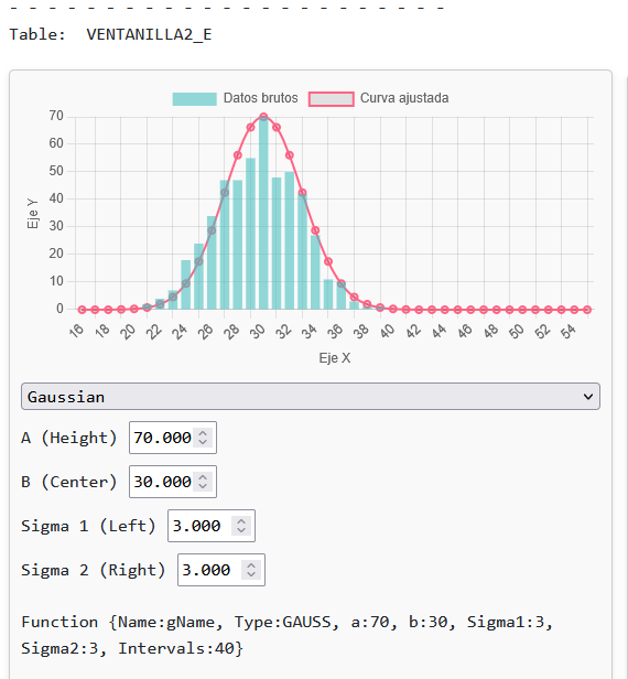
Example:
/* Defining functions */ SYSTEM {TYPE:OPTIONS,Speed:5} Facility {NAME:VENTANILLA1,X:165,Y:184,E_BIN_start:16,E_BIN_SIZE:1,E_BIN_COUNT:40,capacity:3} Facility {NAME:VENTANILLA2,X:384,Y:186,E_BIN_start:16,E_BIN_SIZE:1,E_BIN_COUNT:40,capacity:3} POSITION {NAME:POS1,X:278,Y:381} POSITION {NAME:POS2,X:482,Y:380} Function {name:funGauss, type:"GAUSS", a:1, b:30, sigma1:3.3, sigma2:3.3,intervals:100 } Function {NAME:funValues,type:"VALUES",expression:"RANDOM",VALUES:" 0.0001,0.0000/0.0002,0.0101/0.0004,0.0202/0.0006,0.0303/0.0008,0.0404/ 0.0011,0.0505/0.0015,0.0606/0.0020,0.0707/0.0025,0.0808/0.0032,0.0909/ 0.0039,0.1010/0.0049,0.1111/0.0060,0.1212/0.0073,0.1313/0.0088,0.1414/ 0.0106,0.1515/0.0128,0.1616/0.0152,0.1717/0.0180,0.1818/0.0213,0.1919/ 0.0250,0.2020/0.0293,0.2121/0.0341,0.2222/0.0396,0.2323/0.0458,0.2424/ 0.0527,0.2525/0.0603,0.2626/0.0689,0.2727/0.0783,0.2828/0.0887,0.2929/ 0.1000,0.3030/0.1124,0.3131/0.1258,0.3232/0.1403,0.3333/0.1559,0.3434/ 0.1726,0.3535/0.1904,0.3636/0.2093,0.3737/0.2292,0.3838/0.2501,0.3939/ 0.2720,0.4040/0.2948,0.4141/0.3185,0.4242/0.3429,0.4343/0.3680,0.4444/ 0.3937,0.4545/0.4199,0.4646/0.4464,0.4747/0.4731,0.4848/0.5000,0.4949/ 0.5269,0.5051/0.5536,0.5152/0.5801,0.5253/0.6063,0.5354/0.6320,0.5455/ 0.6571,0.5556/0.6815,0.5657/0.7052,0.5758/0.7280,0.5859/0.7499,0.5960/ 0.7708,0.6061/0.7907,0.6162/0.8096,0.6263/0.8274,0.6364/0.8441,0.6465/ 0.8597,0.6566/0.8742,0.6667/0.8876,0.6768/0.9000,0.6869/0.9113,0.6970/ 0.9217,0.7071/0.9311,0.7172/0.9397,0.7273/0.9473,0.7374/0.9542,0.7475/ 0.9604,0.7576/0.9659,0.7677/0.9707,0.7778/0.9750,0.7879/0.9787,0.7980/ 0.9820,0.8081/0.9848,0.8182/0.9872,0.8283/0.9894,0.8384/0.9912,0.8485/ 0.9927,0.8586/0.9940,0.8687/0.9951,0.8788/0.9961,0.8889/0.9968,0.8990/ 0.9975,0.9091/0.9980,0.9192/0.9985,0.9293/0.9989,0.9394/0.9992,0.9495/ 0.9994,0.9596/0.9996,0.9697/0.9998,0.9798/0.9999,0.9899/1.0000,1.0000/ "} START 500 ;***************************************************** GENERATE 10,0,0,0 {NAME:GEN1,X:91,Y:383} ADVANCE 20,4 {TO:VENTANILLA1} SEIZE VENTANILLA1 ADVANCE 20 + (FN$funValues * 20) ; classic definition RELEASE VENTANILLA1 ADVANCE 20,0 {TO:POS1} ADVANCE 20,0 {TO:VENTANILLA2} SEIZE VENTANILLA2 ADVANCE FN$funGauss ; parameter-based definition ;ADVANCE 2 ; parameter-based definition RELEASE VENTANILLA2 ADVANCE 20,0 {TO:POS2} ENDGENERATE 1 - + Types of distribution functions
The
FUNCTIONcommand allows you to define functions that return numeric values, either through direct calculations or through precomputed distribution tables. These functions are used to simulate variable and realistic behavior in operations such asADVANCE,ASSIGN,TABULATE, etc., and they represent times, quantities, costs, probabilities, and more.In GPSS-Plus, functions can be classified into two broad groups:
1. Functions based on statistical distributions (with a value table)
These functions pre-generate an internal table with a configurable number of points (intervals) and interpolate the result over it. They are ideal for representing random behavior with known patterns. Available types are:
-
GAUSS: Normal distribution (Gaussian bell curve). -
EXP: Decreasing exponential distribution. -
UNIFORM: Uniform (rectangular) distribution. -
TRIANGULAR: Triangular distribution. -
LOGNORMAL: Log-normal distribution, right-skewed. -
FDISTRIBUTION: Lets you define a custom distribution function using a mathematical formula.
2. Direct-calculation functions (no table)
These functions evaluate the result directly, without generating or consulting a table. They are more flexible when you want to work with formulas or with discrete event-count models. They include:
-
POISSON: Generates a random integer according to a Poisson distribution (number of events per interval). -
MATH: Directly evaluates a mathematical expression. It accepts multiple parameters that are substituted by letters (A,B,C, etc.) in order.
Example:
Function {name:funGauss, type:"GAUSS", a:1, b:30, sigma1:3.3, sigma2:3.3,intervals:100 } Function {name:funExp, type:"EXP", b:0, lambda:0.15, intervals:100} Function {name:funUni, type:"UNIFORM", min:20, max:40, intervals:100} Function {name:funTri, type:"TRIANGULAR", min:20, max:40, mode:30, intervals:100} Function {name:funLog, type:"LOGNORMAL", mu:3.4, sigma:0.3, intervals:100} Function {name:funLog2, type:"LOGNORMAL", b:30, spread:5, intervals:100} Function {name:funCus, type:"FDISTRIBUTION", function:"A * Math.sin(B * x)", a:10, b:0.5, min:0, max:10, intervals:100} Function {name:funPoi, type:"POISSON", lambda:3.5} Function {Name:math1, type: math, EXPRESSION:"A * 2 + B"} -
- + Gaussian function
The Gaussian (or normal) distribution represents a bell-shaped curve, where the most likely values are near a central value and extremes are less likely. It is ideal for modeling natural phenomena such as service times, measurement errors, or process durations, where most cases cluster around a mean.
Parameters:
- a: Curve height (visualization only; it does not affect the calculation).
- b: Central value or expected mean of the process.
- sigma1: Spread (standard deviation) to the left of the center.
- sigma2: Spread to the right of the center. It can differ from sigma1 to create asymmetry.
- intervals: Number of segments used to divide the curve. The higher the number, the more precise.
By construction, the distribution will take values approximately between
b - sigma1 * 3andb + sigma2 * 3.This example shows how three service windows with different Gaussian functions produce different distributions of service times:
ADVANCE FN$gfun1 ; symmetric
ADVANCE FN$gfun2 ; right spread
ADVANCE FN$gfun3 ; left spread

Example:
/* Gauss */ SYSTEM {TYPE:OPTIONS,Speed:5} Facility {NAME:VENTANILLA1,X:165,Y:184,E_BIN_start:5,E_BIN_SIZE:1,E_BIN_COUNT:80,capacity:10} Facility {NAME:VENTANILLA2,X:343,Y:185,E_BIN_start:5,E_BIN_SIZE:1,E_BIN_COUNT:80,capacity:10} Facility {NAME:VENTANILLA3,X:535,Y:183,E_BIN_start:5,E_BIN_SIZE:1,E_BIN_COUNT:80,capacity:10} POSITION {NAME:POS1,X:250,Y:381} POSITION {NAME:POS2,X:423,Y:383} POSITION {NAME:POS3,X:566,Y:384} Function {name:gfun1, TYPE:GAUSS, a:1, b:50, sigma1:3.3, sigma2:3.3,intervals:100 } Function {name:gfun2, TYPE:GAUSS, a:1, b:50, sigma1:1.0, sigma2:10.0,intervals:100 } Function {name:gfun3, TYPE:GAUSS, a:1, b:50, sigma1:10.0, sigma2:1.0,intervals:100 } START 500 ;***************************************************** GENERATE 10,0,0,0 {NAME:GEN1,X:91,Y:383} ADVANCE 20,4 {TO:VENTANILLA1} SEIZE VENTANILLA1 ADVANCE FN$gfun1 RELEASE VENTANILLA1 ADVANCE 20,0 {TO:POS1} ADVANCE 20,0 {TO:VENTANILLA2} SEIZE VENTANILLA2 ADVANCE FN$gfun2 RELEASE VENTANILLA2 ADVANCE 20,0 {TO:POS2} ADVANCE 20,0 {TO:VENTANILLA3} SEIZE VENTANILLA3 ADVANCE FN$gfun3 RELEASE VENTANILLA3 ADVANCE 20,0 {TO:POS3} ENDGENERATE 1 - + Exponential function
The exponential distribution is used to model events that occur randomly but with a decreasing probability over time. It is ideal for situations such as waiting times, system failures, or random arrivals where something is most likely to occur early, and becomes less likely the longer it takes.
A classic example: "If you are waiting to be served, it is more likely to happen soon; and each additional minute reduces that probability."
This is not well represented by a uniform distribution (such as
ADVANCE 10,5), but it is by an exponential function, defined with the type:Function {name:efun1, type:"EXP", a:100, b:20, lambda:0.3, intervals:100}Parameters
a: Curve height (visual only; it does not affect the calculation).
b: Base minimum value. This is the point from which the distribution starts.
lambda: Decay rate. The higher the lambda, the faster the decay.
intervals: Number of segments into which the curve is divided (the more, the more precise).
Approximately, 99.9% of the values will lie within the range:
λ = 1 → from b to b + 6.91
λ = 0.5 → from b to b + 13.82
λ = 2 → from b to b + 3.45
Comparative usage example:
Function {Name:efun1, type:"EXP", a:100, b:20, lambda:0.3, intervals:70}
Function {Name:efun2, type:"EXP", a:100, b:20, lambda:0.6, intervals:70}
Function {Name:efun3, type:"EXP", a:100, b:20, lambda:1.0, intervals:70}

ADVANCE FN$efun1 ; slow decay
ADVANCE FN$efun2 ; medium decay
ADVANCE FN$efun3 ; fast decay
Example:
/* Exponential */ SYSTEM {TYPE:OPTIONS, Speed:5} ;=== Facilities with statistical tracking === Facility {NAME:VENTANILLA1,X:165,Y:184,E_BIN_start:5,E_BIN_SIZE:1,E_BIN_COUNT:80,capacity:10} Facility {NAME:VENTANILLA2,X:343,Y:185,E_BIN_start:5,E_BIN_SIZE:1,E_BIN_COUNT:80,capacity:10} Facility {NAME:VENTANILLA3,X:535,Y:183,E_BIN_start:5,E_BIN_SIZE:1,E_BIN_COUNT:80,capacity:10} ;=== Final positions for visualization === POSITION {NAME:POS1, X:250, Y:381} POSITION {NAME:POS2, X:423, Y:383} POSITION {NAME:POS3, X:566, Y:384} ;=== EFunctions with different decay rates === Function {Name:efun1, TYPE:EXP, a:100, b:20, Lambda:0.3, Intervals:70} Function {Name:efun2, TYPE:EXP, a:100, b:20, Lambda:0.6, Intervals:70} Function {Name:efun3, TYPE:EXP, a:100, b:20, Lambda:1.0, Intervals:70} ;=== Simulation start === START 500 ;=== Entity flow through the three service windows === GENERATE 10,0,0,0 {NAME:GEN1, X:91, Y:383} ; WINDOW 1 – Slow decay ADVANCE 20,4 {TO:VENTANILLA1} SEIZE VENTANILLA1 ADVANCE FN$efun1 RELEASE VENTANILLA1 ADVANCE 20,0 {TO:POS1} ; WINDOW 2 – Medium decay ADVANCE 20,0 {TO:VENTANILLA2} SEIZE VENTANILLA2 ADVANCE FN$efun2 RELEASE VENTANILLA2 ADVANCE 20,0 {TO:POS2} ; WINDOW 3 – Fast decay ADVANCE 20,0 {TO:VENTANILLA3} SEIZE VENTANILLA3 ADVANCE FN$efun3 RELEASE VENTANILLA3 ADVANCE 20,0 {TO:POS3} ENDGENERATE 1 - + Log-normal function
What is the log-normal distribution?
A variable follows a log-normal distribution if the logarithm of that variable has a normal distribution. In other words:
“Many small events occur frequently, but it is also possible for some events with very large values to appear, although with low probability.”
Typical cases:
Machine repair time.
Duration of a phone call.
Income (most people earn little, a few earn a lot).
Function {Name:lfunc1, Type:LOGNORMAL, b:30, sigma:0.1}Parameters:
b: The function’s most likely value (the peak of the curve).sigma: Controls the spread of values to the right. The larger the sigma, the wider the distribution’s “tail”.
GPSS-Plus automatically converts these values into the mathematical parameters
μ(log-mean) andσ(standard deviation) to build the log-normal curve.Unlike the Gaussian, the log-normal is not symmetric. It has a long “tail” toward higher values. This behavior matches well with phenomena where extreme values are rare, but possible.
This example shows three log-normal functions with the same curve type, but different dispersion.
Function {Name:lfunc1, Type:LOGNORMAL, b:30, sigma:0.1}   ; narrow curve
Function {Name:lfunc2, Type:LOGNORMAL, b:20, sigma:0.15}  ; medium dispersion
Function {Name:lfunc3, Type:LOGNORMAL, b:40, sigma:0.2}   ; long tail
Example:
/* Log-normal */ SYSTEM {TYPE:OPTIONS, Speed:5} Facility {NAME:VENTANILLA1,X:165,Y:184,E_BIN_start:0,E_BIN_SIZE:1,E_BIN_COUNT:100,capacity:10} Facility {NAME:VENTANILLA2,X:343,Y:185,E_BIN_start:0,E_BIN_SIZE:1,E_BIN_COUNT:100,capacity:10} Facility {NAME:VENTANILLA3,X:535,Y:183,E_BIN_start:0,E_BIN_SIZE:1,E_BIN_COUNT:100,capacity:10} POSITION {NAME:POS1, X:250, Y:381} POSITION {NAME:POS2, X:423, Y:383} POSITION {NAME:POS3, X:566, Y:384} Function {Name:lfunc1, Type: LOGNORMAL, b:30, sigma:0.1} Function {Name:lfunc2, Type: LOGNORMAL, b:20, sigma:0.15} Function {Name:lfunc3, Type: LOGNORMAL, b:40, sigma:0.2} START 500 GENERATE 10,0,0,0 {NAME:GEN1, X:91, Y:383} ; WINDOW 1 – Small dispersion ADVANCE 20,4 {TO:VENTANILLA1} SEIZE VENTANILLA1 ADVANCE FN$lfunc1 RELEASE VENTANILLA1 ADVANCE 20,0 {TO:POS1} ; WINDOW 2 – Medium dispersion ADVANCE 20,0 {TO:VENTANILLA2} SEIZE VENTANILLA2 ADVANCE FN$lfunc2 RELEASE VENTANILLA2 ADVANCE 20,0 {TO:POS2} ; WINDOW 3 – Large dispersion (long tail) ADVANCE 20,0 {TO:VENTANILLA3} SEIZE VENTANILLA3 ADVANCE FN$lfunc3 RELEASE VENTANILLA3 ADVANCE 20,0 {TO:POS3} ENDGENERATE 1 - + Uniform function
The uniform distribution represents maximum uncertainty: all values within a range have exactly the same probability.
"It’s like rolling a perfect die: no number is more likely than another."
This type of distribution is useful when there is no reason to believe some values are more likely than others.

Parameters
Function {Name:ufun1, TYPE:UNIFORM, Min:20, Max:40}-
Min: minimum value the function can take. -
Max: maximum value the function can take.
All values between Min and Max have the same probability.
In the report chart, the curve has the shape of a flat rectangle. The wider the range, the more spread out the distribution will be.
This example compares three uniform distributions with different ranges. All have a rectangular shape, but differ in width and position:
Function {Name:ufun1, TYPE:UNIFORM, Min:20, Max:40}   ; Small range
Function {Name:ufun2, TYPE:UNIFORM, Min:20, Max:60}   ; Wide range
Function {Name:ufun3, TYPE:UNIFORM, Min:30, Max:50}   ; Shifted range
Example:
/* Uniforme */ SYSTEM {TYPE:OPTIONS, Speed:5} Facility {NAME:VENTANILLA1,X:165,Y:184,E_BIN_start:5,E_BIN_SIZE:1,E_BIN_COUNT:80,capacity:10} Facility {NAME:VENTANILLA2,X:343,Y:185,E_BIN_start:5,E_BIN_SIZE:1,E_BIN_COUNT:80,capacity:10} Facility {NAME:VENTANILLA3,X:535,Y:183,E_BIN_start:5,E_BIN_SIZE:1,E_BIN_COUNT:80,capacity:10} POSITION {NAME:POS1, X:250, Y:381} POSITION {NAME:POS2, X:423, Y:383} POSITION {NAME:POS3, X:566, Y:384} Function {Name:ufun1, TYPE:UNIFORM, Min:20, Max:40} Function {Name:ufun2, TYPE:UNIFORM, Min:20, Max:60} Function {Name:ufun3, TYPE:UNIFORM, Min:30, Max:50} START 500 GENERATE 10,0,0,0 {NAME:GEN1, X:91, Y:383} ; WINDOW 1 – Uniform from 20 to 40 ADVANCE 20,4 {TO:VENTANILLA1} SEIZE VENTANILLA1 ADVANCE FN$ufun1 RELEASE VENTANILLA1 ADVANCE 20,0 {TO:POS1} ; WINDOW 2 – Uniform from 20 to 60 ADVANCE 20,0 {TO:VENTANILLA2} SEIZE VENTANILLA2 ADVANCE FN$ufun2 RELEASE VENTANILLA2 ADVANCE 20,0 {TO:POS2} ; WINDOW 3 – Uniform from 30 to 50 ADVANCE 20,0 {TO:VENTANILLA3} SEIZE VENTANILLA3 ADVANCE FN$ufun3 RELEASE VENTANILLA3 ADVANCE 20,0 {TO:POS3} TERMINATE 1 -
- + Triangular function
The triangular distribution lets you define a value’s minimum, maximum, and most likely (mode). It has a triangular shape, where the mode is the most frequent value and the extremes are less likely.
It’s useful when you have an approximate idea of how a process behaves, but not enough data to justify a more complex distribution.
“A delivery usually takes 3 days, but it could take 2 or 5.”
That kind of uncertainty is ideal for a triangular distribution.
Parameters
Function {Name:tfun1, TYPE:TRIANGULAR, Min:20, Max:40, Mode:30}Min: Minimum possible value.Max: Maximum possible value.Mode: Most likely value (peak of the distribution).
This example compares three triangular functions with different peak positions. All share the same range, but produce different distributions:
Function {Name:tfun1, TYPE:TRIANGULAR, Min:20, Max:40, Mode:30} ; Centered peak
Function {Name:tfun2, TYPE:TRIANGULAR, Min:20, Max:40, Mode:25} ; Left-skewed peak
Function {Name:tfun3, TYPE:TRIANGULAR, Min:20, Max:40, Mode:35} ; Right-skewed peak
Example:
/* Triangular */ SYSTEM {TYPE:OPTIONS, Speed:5} Facility {NAME:VENTANILLA1,X:165,Y:184,E_BIN_start:0,E_BIN_SIZE:1,E_BIN_COUNT:80,capacity:10} Facility {NAME:VENTANILLA2,X:343,Y:185,E_BIN_start:0,E_BIN_SIZE:1,E_BIN_COUNT:80,capacity:10} Facility {NAME:VENTANILLA3,X:535,Y:183,E_BIN_start:0,E_BIN_SIZE:1,E_BIN_COUNT:80,capacity:10} POSITION {NAME:POS1, X:250, Y:381} POSITION {NAME:POS2, X:423, Y:383} POSITION {NAME:POS3, X:566, Y:384} Function {Name:tfun1, TYPE:TRIANGULAR, Min:20, Max:40, Mode:30} Function {Name:tfun2, TYPE:TRIANGULAR, Min:20, Max:40, Mode:25} Function {Name:tfun3, TYPE:TRIANGULAR, Min:20, Max:40, Mode:35} START 500 GENERATE 10,0,0,0 {NAME:GEN1, X:91, Y:383} ; WINDOW 1 – Centered triangle ADVANCE 20,4 {TO:VENTANILLA1} SEIZE VENTANILLA1 ADVANCE FN$tfun1 RELEASE VENTANILLA1 ADVANCE 20,0 {TO:POS1} ; WINDOW 2 – Triangle with the peak to the left ADVANCE 20,0 {TO:VENTANILLA2} SEIZE VENTANILLA2 ADVANCE FN$tfun2 RELEASE VENTANILLA2 ADVANCE 20,0 {TO:POS2} ; WINDOW 3 – Triangle with the peak to the right ADVANCE 20,0 {TO:VENTANILLA3} SEIZE VENTANILLA3 ADVANCE FN$tfun3 RELEASE VENTANILLA3 ADVANCE 20,0 {TO:POS3} ENDGENERATE 1 - + Poisson function
The Poisson distribution models the number of events that occur in a fixed time interval, provided that:
-
Events occur independently.
-
The average rate of occurrence (λ) is constant.
When should you use Poisson?
-
Number of calls per minute in a call center.
-
Customer arrivals to a store.
-
Manufacturing defects per day.
Parameter:
λ(lambda): the expected mean number of events per interval.For example, if λ = 3, on average there will be 3 events per unit of time, although there can be 2, 4, 0, etc. The variability is part of the distribution.
Relationship with the exponential distribution
-
Poisson counts how many events occur.
-
Exponential measures the time between events.
Both are controlled by the same parameter λ, and they are complementary:
Poisson(λ): Number of events per interval λ
Exponential(λ): Time between consecutive events 1 / λWhat does this example show?
A visual comparison of both distributions for 3 different values of λ:
Function {Name:fPoisson1, TYPE:POISSON, LAMBDA:X$LAMBDA1}
Function {Name:fPoisson2, TYPE:POISSON, LAMBDA:X$LAMBDA2}
Function {Name:fPoisson3, TYPE:POISSON, LAMBDA:X$LAMBDA3}

Function {Name:fexp1, TYPE:EXP, LAMBDA:X$LAMBDA1, b:0}
Function {Name:fexp2, TYPE:EXP, LAMBDA:X$LAMBDA2, b:0}
Function {Name:fexp3, TYPE:EXP, LAMBDA:X$LAMBDA3, b:0}
The results are shown as dynamic text using the running mean:
Converges to λ = 3.0 → Mean ≈ 3.0
Converges to λ = 0.25 → Mean ≈ 0.25

Exp = 1 / λ = 0.333 → Mean ≈ 0.333
This simulation helps you see how:
-
Poisson stabilizes the event count toward λ.
-
Exponential stabilizes the time between events toward 1 / λ.

Example:
/* Poisson */ SYSTEM {TYPE:OPTIONS,Speed:5} Graphic {NAME:pText1,Type:TEXT,X:309,Y:281,Text:"Mean1"} Graphic {NAME:pText2,Type:TEXT,X:309,Y:238,Text:"Mean2"} Graphic {NAME:pText3,Type:TEXT,X:308,Y:198,Text:"Mean3"} Graphic {NAME:eText1,Type:TEXT,X:506,Y:280,Text:"Exp1"} Graphic {NAME:eText2,Type:TEXT,X:506,Y:238,Text:"Exp2"} Graphic {NAME:eText3,Type:TEXT,X:504,Y:196,Text:"Exp3"} POSITION {NAME:POS1,X:598,Y:395} INITIAL contador,0 INITIAL LAMBDA1,1/4 INITIAL iLAMBDA1,round(1/X$LAMBDA1,3) INITIAL pTotal1,0 INITIAL eTotal1,0 INITIAL LAMBDA2,3/4 INITIAL iLAMBDA2,round(1/X$LAMBDA2,3) INITIAL pTotal2,0 INITIAL eTotal2,0 INITIAL LAMBDA3,3 INITIAL iLAMBDA3,round(1/X$LAMBDA3,3) INITIAL pTotal3,0 INITIAL eTotal3,0 Function {Name:fPoisson1, TYPE:POISSON, LAMBDA:X$LAMBDA1} Function {Name:fPoisson2, TYPE:POISSON, LAMBDA:X$LAMBDA2} Function {Name:fPoisson3, TYPE:POISSON, LAMBDA:X$LAMBDA3} Function {Name:fexp1, TYPE:EXP, LAMBDA:X$LAMBDA1, b:0} Function {Name:fexp2, TYPE:EXP, LAMBDA:X$LAMBDA2, b:0} Function {Name:fexp3, TYPE:EXP, LAMBDA:X$LAMBDA3, b:0} START 2000 ;***************************************************** GENERATE 2,0,0,0 {NAME:GEN1,X:218,Y:395} SAVEVALUE contador,X$contador + 1 ; --- Accumulation Poisson --- SAVEVALUE pTotal1,X$pTotal1 + FN$fPoisson1 SAVEVALUE pMedia1, X$pTotal1 / X$contador SAVEVALUE pMediaRound1, round(X$pMedia1,3) SAVEVALUE pTotal2,X$pTotal2 + FN$fPoisson2 SAVEVALUE pMedia2, X$pTotal2 / X$contador SAVEVALUE pMediaRound2, round(X$pMedia2,3) SAVEVALUE pTotal3,X$pTotal3 + FN$fPoisson3 SAVEVALUE pMedia3, X$pTotal3 / X$contador SAVEVALUE pMediaRound3, round(X$pMedia3,3) ; --- Accumulation Exponential --- SAVEVALUE eTotal1,X$eTotal1 + FN$fexp1 SAVEVALUE eMedia1, X$eTotal1 / X$contador SAVEVALUE eMediaRound1, round(X$eMedia1,3) SAVEVALUE eTotal2,X$eTotal2 + FN$fexp2 SAVEVALUE eMedia2, X$eTotal2 / X$contador SAVEVALUE eMediaRound2, round(X$eMedia2,3) SAVEVALUE eTotal3,X$eTotal3 + FN$fexp3 SAVEVALUE eMedia3, X$eTotal3 / X$contador SAVEVALUE eMediaRound3, round(X$eMedia3,3) move {name:pText1,text:"Converges to Lambda = X$LAMBDA1 --> X$pMediaRound1"} move {name:pText2,text:"Converges to Lambda = X$LAMBDA2 --> X$pMediaRound2"} move {name:pText3,text:"Converges to Lambda = X$LAMBDA3 --> X$pMediaRound3"} move {name:eText1,text:"Exp = 1/X$LAMBDA1 = X$iLAMBDA1 --> X$eMediaRound1"} move {name:eText2,text:"Exp = 1/X$LAMBDA2 = X$iLAMBDA2 --> X$eMediaRound2"} move {name:eText3,text:"Exp = 1/X$LAMBDA3 = X$iLAMBDA3 --> X$eMediaRound3"} ADVANCE 30,10 {TO:POS1} ENDGENERATE 1 -
- + FDISTRIBUTION functions
Custom distributions
The
FDISTRIBUTIONtype lets you define fully customized distribution functions using a mathematical expression, without being limited to predefined formulas such asGAUSS,EXPorTRIANGULAR.These functions internally generate a distribution table by evaluating a mathematical expression over a given range. This is ideal for representing non-standard distributions or variants of the classic ones.
How does it work?
GPSS-Plus builds a distribution table based on:
-
A mathematical expression that defines the shape of the function (a bell, a triangle, etc.)
-
A value range (
min,max) over which that function is evaluated -
A number of
intervalsthat determines the table resolution -
Optional parameters (
A,B,C...) that you can use inside the formula
Once the table is built, the function behaves like any other distribution: a random value is drawn, the table is consulted, and the corresponding result is returned.
Syntax:
Function {
  Name: name,
  Type: FDISTRIBUTION,
  Expression: "formula",
  min: minValue,
  max: maxValue,
  intervals: count,
  A: value, B: value, ...
}
Example 1: Custom Gaussian distribution
Function {
  Name:gauss1,
  Type: FDISTRIBUTION,
  EXPRESSION: "(1 / (A * SQRT(2 * PI))) * EXP(-0.5 * ((X - B) / A)^2)",
  A: 2.3,
  B: 30,
  min: B - (3 * A),
  max: B + (3 * A),
  intervals: 100
}
This example creates a bell-shaped function centered at 30, with dispersion 2.3. It is equivalent to a classic Gaussian, but fully configurable.
Example 2: Triangular distribution defined by formula
Function {
  Name:tri1,
  Type: FDISTRIBUTION,
  EXPRESSION: "(1 / C) * (1 - ABS((X - B) / (C / 2)))",
  B: 25, C: 30,
  min: B - C / 2,
  max: B + C / 2,
  intervals: 100
}
This function generates a triangular distribution with its peak at 25, total width 30, and base [10, 40].
Technical details:
-
The variable
Xis the horizontal axis (domain). -
The function is evaluated
intervalstimes betweenminandmax. -
The integral is automatically normalized so it behaves like a probability distribution.
-
All parameters (
A,B,C, etc.) can be expressions.
Example:
/* FDistribution */ SYSTEM {TYPE:OPTIONS,Speed:5} Facility {NAME:VENTANILLA1,X:244,Y:190,E_BIN_start:5,E_BIN_SIZE:1,E_BIN_COUNT:80,capacity:20} Facility {NAME:VENTANILLA2,X:412,Y:188,E_BIN_start:5,E_BIN_SIZE:1,E_BIN_COUNT:80,capacity:20} POSITION {NAME:POS1,X:200,Y:387} POSITION {NAME:POS2,X:341,Y:381} POSITION {NAME:POS3,X:507,Y:380} ;GAUSSIAN Function {Name:tName1, type: FDISTRIBUTION, EXPRESSION:"(1 / (A * SQRT(2 * PI))) * EXP(-0.5 * ((X - B) / A)^2)", b:30, a: 2.3, min:B - (3 * A), max:B + (3 * A),intervals:100} ; TRIANGULAR B: center of the range C: total width of the range Function {Name:tName2, A:0, B:25, C:30, D:0, type: FDISTRIBUTION, EXPRESSION:"(1 / C) * (1 - ABS((X - B) / (C / 2)))", min:B - C/2, max:B + C/2, intervals:100} START 1000 ;***************************************************** GENERATE 2,0,0,0 {NAME:GEN1,X:56,Y:319} ADVANCE 20,0 {TO:POS1} ADVANCE 30,10 {TO:VENTANILLA1} SEIZE VENTANILLA1 ADVANCE FN$tName1 RELEASE VENTANILLA1 ADVANCE 20,0 {TO:POS2} ADVANCE 20,10 {TO:VENTANILLA2} SEIZE VENTANILLA2 ADVANCE FN$tName2 RELEASE VENTANILLA2 ADVANCE 20,0 {TO:POS3} ENDGENERATE 1 -
- + MATH functions
Custom mathematical formulas
The
MATHtype lets you define functions that are evaluated as direct mathematical formulas, without using distributions or precomputed value tables. They are useful when the value we need depends on variables deterministically, or on an algebraic expression.This type of function does not generate randomness. It simply takes the parameters in order, substitutes them into the expression, and returns the result.
Syntax:
Function {Name:name, Type:MATH, Expression:"A + B * C"}Name: identifier name of the function.Type: must beMATH.Expression: formula to evaluate, using uppercase letters as variables (A, B, C...). These letters represent the parameters passed in order.
How do you call a
MATHfunction?It is used like any
FN$function, but with parameters in parentheses:FN$(name, value_A, value_B, ...)
Example:
/*

  	 	Math

*/
Graphic {NAME:Text1,Type:TEXT,X:370,Y:312,Text:"Hello"}

Function {Name:math1, type: MATH, EXPRESSION:"A * 2 + B"}

START 1
;*****************************************************
GENERATE 1,0,0,1 {NAME:GEN1,X:56,Y:319}

assign AAA,4
assign BBB,6

move {name:Text1,text:"Result: FN$(math1,P$AAA,P$BBB)"}

ENDGENERATE 1
- + Defining functions
- + Season 10: Continuous Systems
- + Continuous system within the discrete
So far we have seen how GPSS-Plus is, in its essence, a discrete event simulation engine. However, it is also capable of simulating continuous systems—those in which changes occur gradually over time.
What is a continuous system?
A continuous system is one where values change without interruptions. For example:
- The level of a tank being filled.
- The temperature of a furnace being heated.
- The velocity of a car accelerating smoothly.
In these cases, there are no discrete "jumps" like those in a queue or a customer entering or leaving. The change happens progressively.
How to simulate that in a discrete environment?
The answer is: cheating, but intelligently. Instead of simulating a constant and fluid change, we divide it into small time steps, fast enough so that it looks continuous.
It is like cinema: each frame is a static image, but when played at 24 frames per second, we perceive motion.How is this done in GPSS-Plus?
With key adjustments:
SYSTEM {type:OPTIONS, TIME_DECIMALS:1, SPEED:5}TIME_DECIMALS:1indicates that time is measured with one decimal place (0.1).SPEED:5sets the system update to a medium speed. From 0 (pause) to 10 (maximum speed). A medium speed (5) means that 10 AC1 instants take approximately 1 second. WithSPEED:2, 1 second is roughly equivalent to 1 AC1.
The engine remains discrete. Time does not advance on its own; it advances when an entity is serviced or an event is triggered. What we do is generate many small events in rapid succession.
Example: Filling a tank
We are going to fill a tank with a variable flow rate (for example, following a sine function to make it more dynamic).
To do this, we use a timer, which launches a block of code every 0.1 units of time. It does not generate transactions or statistics: it just executes.
SYSTEM {TYPE:ON_TIMER, TRIGGER:filling, INTERVAL: 0.1}Each time the
PROCEDUREis triggered, we will:- Calculate a flow rate based on an oscillating function, previously defined with
FUNCTION TYPE:MATH. - Add that flow to the current tank level.
- Visually update the level.
- Display the value on the screen.
- Stop the simulation if the tank becomes full.
In this case, each cycle calculated the flow rate and added it to the level using a simple formula:
SAVEVALUE level, X$level + X$flow * 0.1
This method is called the Euler method, and it is the simplest form of numerical integration.
It estimates that during the time interval between AC1$ and AC1$ + 0.1, the tank will fill by an amount equal to the flow rate at instant AC1$ multiplied by the 0.1 interval.
In the next step, it will perform the same calculation again using the new flow rate value at that instant. And so on, adding small amounts as if it were a sum of rectangles: that is, in essence, an integral.
Example:
/* Continuous system within the discrete */ SYSTEM {TYPE:PRE_RUN,TRIGGER:PRE_RUN} SYSTEM {type:OPTIONS, TIME_DECIMALS:1, SPEED:5} SYSTEM {TYPE:ON_TIMER, TRIGGER:filling, INTERVAL: 0.1} Graphic {NAME:alert,Type:TEXT,X:291,Y:342,Text:"alert"} Function {Name:fcFlow, Type:Math, Expression:"0.6 + SIN(A) * 4"} INITIAL level, 0 INITIAL flow, 1.2 INITIAL phase, 0 INITIAL constant, 0.6 include ./library_graphics/speedometer.lib START 100 PROCEDURE PRE_RUN assign config,{title:"Tank" ,x:100,y:60 ,width:100 ,height:180 ,min_value: 0 ,max_value: 100 ,"color":"#ff0000"} call tank.speedometer.init,V$config assign config,{title:"Flow Rate" ,x:300,y:60 ,width:100 ,height:180 ,min_value: -10 ,max_value: 10 ,"color":"orange"} call flow.speedometer.init,V$config TERMINATE_VE ENDPROCEDURE PROCEDURE filling ; Oscillate flow rate as a function of simulated time SAVEVALUE flow, FN$(fcFlow,X$fase) ; Increment the phase smoothly SAVEVALUE phase, X$fase + 0.1 ; Add flow to the level, according to the time interval SAVEVALUE level, X$level + X$flow * 0.1 ; Rounded values for display ASSIGN tFlow, round(X$flow, 2) ASSIGN tLevel, round(X$level, 2) CALL tank.speedometer.set, P$tLevel CALL flow.speedometer.set, P$tFlow ; Status visualization IF (X$level>=100) MOVE {name:alert, text:"TANK FULL!"} STOP ELSE MOVE {name:alert, text:"Level: P$tLevel - Flow: P$tFlow"} ENDIF TERMINATE ENDPROCEDURE 1 - + PLOT data collection
In the previous chapter we saw how GPSS-Plus can simulate apparently continuous behaviors by using
TIMERsand very small time steps. We observed, for example, how a tank was filled on screen, simulating a constant process.Now we go one step further:
We are not only going to see what happens… we are going to record it and automatically plot it for later analysis.Because in many cases, observing motion is not enough: we need a curve, a graph, a historical record of the behavior.
For that purpose, GPSS-Plus provides a data tracing system:PLOTTERandPLOTPLOTTER {}: declares a graphical table where values will be stored.PLOT: adds a point to that table, using the current time or another variable as the X axis.
Each added point is like a system “frame”, and when the simulation ends, GPSS-Plus draws a curve using all recorded points.
Usage example
In our case, we will record:
PLOTTER {NAME:thePlot, Y_0:level, Y_1:flow, X:TIME_AC1}This means:
- We will plot two value series:
levelandflow. - The horizontal axis (X) will be time (
AC1$), referenced asTIME_AC1.
To add points at each instant:
PLOT thePlot, X$level, X$flow
This is executed inside the
PROCEDURE, on every call, gradually building the process history.“LEVEL is obtained by accumulating FLOW. The system simulates a continuous integration.”
“Each point corresponds to an instant automatically generated by the TIMER.”
Example:
/* PLOT data collection */ SYSTEM {TYPE:PRE_RUN,TRIGGER:PRE_RUN} SYSTEM {type:OPTIONS, TIME_DECIMALS:1, SPEED:5} SYSTEM {TYPE:ON_TIMER, TRIGGER:filling, INTERVAL: 0.1} PLOTTER {NAME:thePlot, Y_0:level, Y_1:flow, X:TIME_AC1} Graphic {NAME:warning,Type:TEXT,X:291,Y:342,Text:"warning"} Function {Name:fcFlow, Type:Math, Expression:"0.6 + SIN(A) * 4"} INITIAL level, 0 INITIAL flow, 1.2 INITIAL phase, 0 include ./library_graphics/speedometer.lib START 100 PROCEDURE PRE_RUN assign config,{title:"Tank" ,x:100,y:60 ,width:100 ,height:180 ,min_value: 0 ,max_value: 100 ,"color":"#ff0000"} call tank.speedometer.init,V$config assign config,{title:"Flow" ,x:300,y:60 ,width:100 ,height:180 ,min_value: -10 ,max_value: 10 ,"color":"orange"} call flow.speedometer.init,V$config TERMINATE_VE ENDPROCEDURE PROCEDURE filling ; Oscillate flow as a function of simulated time SAVEVALUE flow, FN$(fcFlow,X$phase) ; Increase phase SAVEVALUE phase, X$phase + 0.1 ; Add flow to the level SAVEVALUE level, X$level + X$flow * 0.1 ; Record data into the plotter PLOT thePlot, X$level, X$flow ; Display rounded values ASSIGN tFlow, round(X$flow, 2) ASSIGN tLevel, round(X$level, 2) ; Update visual indicators CALL tank.speedometer.set, P$tLevel CALL flow.speedometer.set, P$tFlow IF (X$level>=100) MOVE {name:warning, text:"TANK FULL!"} STOP ELSE MOVE {name:warning, text:"Level: P$tLevel - Flow: P$tFlow"} ENDIF TERMINATE ENDPROCEDURE 1 - + Improving results with INTEGRATE
In previous chapters we saw how GPSS-Plus can simulate systems with an apparently continuous behavior thanks to frequent execution of timed procedures (
TIMER) and the use ofSAVEVALUEto accumulate values such as filling a tank.Up to now we used a simple formula to simulate the filling:
SAVEVALUE level, X$level + X$flow * 0.1
This method is effective, but basic. It assumes the flow is constant during each time interval, which is not entirely true if the flow changes rapidly, for example with a sine function as in this case.
And when we talk about interval, here we are talking about that "0.1". SIN(0) is not the same as SIN(0.1). And if we want a more accurate estimate of the average value, it would probably be better to use
SIN(0.05), i.e., the midpoint of the interval.What happens if the flow varies during the time step?
When the value you are accumulating changes within the same interval, the system is not perfectly exact: you are adding an approximate average value, not the real one.
To improve this, GPSS-Plus includes the
INTEGRATEblock, which uses a numerical integration method called fourth-order Runge-Kutta (RK4) to compute a much more accurate estimate.What does INTEGRATE do?
INTEGRATE { EXPRESSION: "SIN(T) + 2", DT: 0.1, SAVEVALUE: flow_RK4 }This block:
-
Evaluates the expression at four key points of the interval: at the start (
X), twice at the midpoint (X + DT/2), and at the end (X + DT). -
Applies the fourth-order Runge-Kutta (RK4) method, combining those values with specific weights to accurately estimate how the function varies over that segment.
-
Stores the result in the indicated
SAVEVALUE, as a better estimate of the average value of the expression over that interval.
The resulting value will be a better estimate of the mean flow in that time interval, and we can use it to fill the tank more accurately.
Comparing the traditional method (Euler) and RK4
We will build an example that uses both methods in parallel:
flow: using the simple methodflow_RK4: using RK4 numerical integrationlevel: accumulated with the classic flowlevel_RK4: accumulated with the RK4 flow
In addition, we will plot the 4 curves using
PLOTTERto visually compare the results.What will you see in the plot?
level_RK4rises slightly more smoothly and a bit faster thanlevel, because it accounts for the fact that the flow grows within the interval.flow_RK4matches peaks and valleys better thanflow, which only evaluates a single point.The white line on screen (RK4 level) goes a bit ahead of the blue line (simple level).
When is it valid to use RK4?
The fourth-order Runge-Kutta (RK4) method, implemented by the
INTEGRATEblock in GPSS-Plus, is a numerical algorithm designed to solve ordinary differential equations of the form:dy/dt = f(t)
And it does so assuming that the function
f(t)is continuous and smooth over the interval being integrated.But… GPSS-Plus is a discrete-event system
This means there are many variables (
X$level,X$entitiesInQueue,X$facility, etc.) that can change abruptly, without continuity or smoothness.Those changes depend on events that fire when other entities arrive, seize resources, or finish.
Therefore:
You should not use INTEGRATE with expressions that depend on discrete system elements.
INTEGRATE with RK4 is a powerful and accurate tool, as long as it is used with purely mathematical functions. It is not a magical simulation of the future: it is an intelligent estimator for a well-defined function.
Example:
/* Improving results with INTEGRATE */ SYSTEM {type:OPTIONS, TIME_DECIMALS:1, SPEED:5} SYSTEM {TYPE:ON_TIMER, TRIGGER:filling, INTERVAL: 0.1} PLOTTER {NAME:thePlot, Y_0:level, Y_1:flow,X:TIME_AC1} PLOTTER {NAME:thePlot_RK4, Y_0:level, Y_1:flow,X:TIME_AC1} PLOTTER {NAME:thePlot_ALL, Y_0:level, Y_1:flow, Y_2:level_RK4, Y_3:flow_RK4,X:TIME_AC1} Graphic {NAME:warning,Type:TEXT,X:291,Y:342,Text:"warning"} Graphic {NAME:warning_RK4,Type:TEXT,X:291,Y:302,Text:"Warning2"} Graphic {NAME:Cube1,Type:LINE,POINTS:"[100,100],[100,500],[200,500],[200,100]" , Close:1 , color:#00FFFF , Fcolor:#FFFFFF} Graphic {NAME:Line1,Type:LINE,fcolor:#FF6666, X1:102,Y1:100,X2:198,Y2:100} Graphic {NAME:Line_RK4,Type:LINE,color:#333300, X1:98,Y1:100,X2:202,Y2:100} INITIAL level, 0 INITIAL flow, 1.2 INITIAL level_RK4, 0 INITIAL flow_RK4, 1.2 INITIAL phase, 0 INITIAL constant, 0.6 START 100 ;***************************************************** PROCEDURE filling ; Oscillate flow as a function of simulated time SAVEVALUE flow, X$constant + SIN(X$phase) * 4 ; Smoothly increase the phase SAVEVALUE phase, X$phase + 0.1 ; Continuous integration of the level INTEGRATE { EXPRESSION: "X$constant + SIN(T) * 4", METHOD: RK4, DT: 0.1, SAVEVALUE: flow_RK4 } SAVEVALUE level, X$level + X$flow * 0.1 SAVEVALUE level_RK4, X$level_RK4 + X$flow_RK4 * 0.1 PLOT thePlot,X$level,X$flow PLOT thePlot_RK4,X$level_RK4,X$flow_RK4 PLOT thePlot_ALL,X$level,X$flow,X$level_RK4,X$flow_RK4 MOVE {NAME:Line1, X1:98,Y1:(100+X$level*4) ,X2:202,Y2:(100+X$level*4)} MOVE {NAME:Line_RK4, X1:98,Y1:(100+X$level_RK4*4) ,X2:202,Y2:(100+X$level_RK4*4)} ASSIGN tFlow, round(X$flow, 2) ASSIGN tLevel, round(X$level, 2) ASSIGN tFlow_RK4, round(X$flow_RK4, 2) ASSIGN tLevel_RK4, round(X$level_RK4, 2) ; State display IF (X$level>=100) MOVE {name:warning, text:"TANK FULL!"} stop ELSE MOVE {name:warning, text:"Level: P$tLevel - Flow: P$tFlow"} MOVE {name:warning_RK4, text:"Level: P$tLevel_RK4 - Flow: P$tFlow_RK4"} ENDIF TERMINATE ENDPROCEDURE 1 -
- + Constant acceleration motion
This example shows how to simulate the motion of a vehicle on a circular track using constant acceleration. It is a first step toward building simple physical models, such as those used in basic game engines or mechanical simulations.
What is being simulated?
- The car starts from rest (velocity 0).
- A constant positive acceleration is applied until a maximum speed is reached (4 radians per second).
- Once this limit is reached, acceleration is reversed so the car decelerates smoothly down to a minimum speed (0.2 rad/s).
- Then it accelerates again, repeating the cycle.
How is it calculated?
The
INTEGRATEblock is used to accumulate acceleration over time:INTEGRATE {EXPRESSION: X$aceleracion, DT: 0.01, SAVEVALUE: deltaVel}Since acceleration is constant:
deltaVel = X$aceleracion * 0.01
This increment is then accumulated into the velocity:
SAVEVALUE velocidad, X$velocidad + X$deltaVel
Visual and graphical result
- The car moves smoothly around the circular track, accelerating and braking.
- The resulting plot (
PLOTTER) shows two curves:- Acceleration: a square wave switching between positive and negative values.
- Velocity: a triangular wave responding to the acceleration.
This behavior is typical of a basic speed control system and serves as a foundation for variable acceleration, friction, or adaptive control models.
Example:
/* Constant acceleration motion */ SYSTEM {type:OPTIONS, TIME_DECIMALS:2, SPEED:5} SYSTEM {TYPE:ON_TIMER, TRIGGER:moverCoche, INTERVAL: 0.01} ; --- Initial variables --- INITIAL velocidad, 0.0 ; Angular velocity INITIAL angulo, 0 ; Angular position (radians) INITIAL aceleracion, 0.01 ; Constant angular acceleration INITIAL radio, 200 ; Circular track radius ; --- Graphic elements --- Graphic {NAME:txtVel, Type:TEXT, X:510, Y:120, TEXT:"Velocity:"} Graphic {NAME:coche, Type:LINE, X1:-10, Y1:-10, X2:-10, Y2:10, X3:10, Y3:10, X4:10, Y4:-10, COLOR:#FF0000, close:1} Graphic {NAME:pista, Type:ARC, X:300, Y:300, RADIUS:X$radio, CLOSE:0, COLOR:#999999} ; --- Evolution plot --- PLOTTER {NAME:curva, Y_0:aceleracion, Y_1:velocidad, X:TIME} START 500 ; --- Motion procedure --- PROCEDURE moverCoche IF (X$velocidad >= 4) SAVEVALUE aceleracion, -0.1 ; Start braking ENDIF IF (X$velocidad <= 0.2) SAVEVALUE aceleracion, 0.1 ; Accelerate again ENDIF ; Compute velocity increment INTEGRATE {EXPRESSION: X$aceleracion, DT: 0.01, SAVEVALUE: deltaVel} ; Accumulate velocity SAVEVALUE velocidad, X$velocidad + X$deltaVel ; Advance angle using velocity SAVEVALUE angulo, X$angulo + X$velocidad * 0.05 ; Compute position ASSIGN rad, X$angulo ASSIGN posX, 300 + X$radio * COS(P$rad) ASSIGN posY, 300 + X$radio * SIN(P$rad) MOVE {NAME:coche, X:P$posX, Y:P$posY} ASSIGN tVel, round(X$velocidad, 2) MOVE {NAME:txtVel, TEXT: "Velocity: P$tVel rad/s"} PLOT curva, X$aceleracion, X$velocidad TERMINATE ENDPROCEDURE - + Variable acceleration motion
This example extends the circular motion simulation by allowing the vehicle acceleration to evolve dynamically over time.
Instead of switching abruptly between fixed acceleration values, the system now adjusts acceleration gradually, producing behavior closer to real vehicles: slow acceleration and sharper braking.
What is modeled?
- Progressive acceleration when starting from rest.
- Stronger braking at higher speeds.
- Continuous circular motion.
- Real-time visualization of position and velocity.
- Plots showing the evolution of acceleration and velocity.
Key components
acceleration: current angular acceleration.deltaA: incremental change applied to acceleration.INTEGRATE: computes velocity change from acceleration.velocity: smoothly varying angular speed.angle: angular position driving the motion.PLOTTER: records acceleration and velocity over time.
Acceleration control logic
- Acceleration increases slowly while speed is low.
- When acceleration exceeds a threshold, its growth reverses, producing braking.
- Once velocity reaches zero, the system resets and accelerates again.
The resulting motion resembles a realistic drive cycle with smooth acceleration and sharper deceleration.
Visual outcome
- Acceleration follows a sawtooth-like pattern.
- Velocity exhibits smooth oscillations.
- The car changes color: green while accelerating, red while braking.
Example:
/* Variable acceleration motion */ SYSTEM {type:OPTIONS, TIME_DECIMALS:2, SPEED:6} SYSTEM {TYPE:ON_TIMER, TRIGGER:moverCar, INTERVAL: 0.1} ; --- Initial variables --- INITIAL velocity, 0.0 ; Angular velocity INITIAL angle, 0 ; Angular position (radians) INITIAL acceleration, 0.01 ; Angular acceleration INITIAL radius, 200 ; Circular track radius INITIAL deltaA, 0.0002 ; --- Graphics --- Graphic {NAME:txtVel, Type:TEXT, X:510, Y:120, TEXT:"Velocity:"} Graphic {NAME:car, Type:LINE, X1:-10, Y1:-10, X2:-10, Y2:10, X3:10, Y3:10, X4:10, Y4:-10, COLOR:green, close:1} Graphic {NAME:track, Type:ARC, X:300, Y:300, RADIUS:X$radius, CLOSE:0, COLOR:#999999} ; --- Evolution plot --- PLOTTER {NAME:curve, Y_0:acceleration, Y_1:velocity, X:TIME} START 500 PROCEDURE moverCar ;------------------------------- ; SMOOTH ACCELERATION CONTROL ;------------------------------- ; If acceleration is too high, reduce it smoothly IF (X$acceleration > 0.04) SAVEVALUE deltaA, -0.003 SAVEVALUE acceleration, 0.04 MOVE {name:car, color:red} ENDIF ; If velocity reaches zero, reset and start accelerating again IF (X$velocity <= 0.0) SAVEVALUE deltaA, 0.0002 SAVEVALUE acceleration, 0 SAVEVALUE velocity, 0.0 MOVE {name:car, color:green} ENDIF ;--------------------------------- ; UPDATE VELOCITY AND POSITION ;--------------------------------- ; Gradually modify acceleration SAVEVALUE acceleration, X$acceleration + X$deltaA ; Integrate acceleration to obtain velocity increment INTEGRATE {EXPRESSION: X$acceleration, DT: 0.1, SAVEVALUE: deltaVel} SAVEVALUE velocity, X$velocity + X$deltaVel ; Update angular position SAVEVALUE angle, X$angle + X$velocity * 0.1 ;-------------------------------- ; COMPUTE POSITION AND MOVE CAR ;-------------------------------- ASSIGN rad, X$angle ASSIGN posX, 300 + X$radius * COS(P$rad) ASSIGN posY, 300 + X$radius * SIN(P$rad) MOVE {NAME:car, X:P$posX, Y:P$posY} ;-------------------------- ; DISPLAY STATE AND PLOTS ;-------------------------- ASSIGN tVel, round(X$velocity, 2) ASSIGN tAcc, round(X$acceleration, 4) MOVE {NAME:txtVel, TEXT:"Velocity: P$tVel rad/s\nAcceleration: P$tAcc"} ; Plot data for analysis PLOT curve, X$acceleration, X$velocity TERMINATE ENDPROCEDURE - + Hybrid simulation
In the previous chapters we simulated a tank fill using continuous functions, recorded its evolution with
PLOTTER, and improved accuracy with numerical integration (INTEGRATE, RK4). Now we combine all of that into a realistic hybrid system where continuous and discrete logic coexist.Example: solar station with users connected
This model represents a hybrid system where:
- There is a solar energy source (continuous model)
- There are discrete users who arrive, decide whether they need to charge, and connect if needed
Continuous part: solar generation
Solar input is modeled as a sinusoid that simulates the day cycle: it oscillates smoothly from 0 to 1.5 over 1440 minutes (24 hours). Each time unit represents one minute, and each timer tick adds energy to the system battery.
INTEGRATE {
  EXPRESSION: "0.75 + 0.75 * SIN((T / 1440) * 6.2832)",
  DT: 1,
  SAVEVALUE: solarFlow
}
The result is accumulated into
batteryLevelwith a maximum cap of 100. APLOTTERrecords both battery level and solar flow every cycle, producing a full-day evolution curve in the report.Discrete part: users requesting charge
Users arrive using
GENERATE. Each one decides whether to charge using a Poisson-based decision function:Function {Name:chargeDecision, TYPE:POISSON, LAMBDA:1/4}If they decide to charge, they move to the charger resource (
RESTROOM), wait there, and are released automatically viaWAKEonce they reach the required charge level (requiredCharge).How both worlds are coordinated
Every time
solarCycleruns:- Solar flow is updated (continuous)
- The system battery is recharged with that flow
- All users currently connected to the charger are iterated (
FOREACH ... IN_RESOURCE) and receive energy if available - Fully charged users are released using
WAKE
Visually, the model shows a battery tank level, an arc representing current solar intensity, and a plot of the recorded evolution.
Conclusion
This is a continuous/discrete hybrid model: a continuous environmental evolution (solar generation) combined with discrete arrivals, decisions, and resource occupancy (users charging). This structure is typical in energy systems, shared infrastructure, and any scenario with intermittent production and variable demand.
Example:
/*

 Hybrid simulation

*/
SYSTEM {type:OPTIONS, TIME_DECIMALS:0, SPEED:5}                 ; Integer time units (no decimals) and slow visual simulation
SYSTEM {TYPE:ON_TIMER, TRIGGER:solarCycle, INTERVAL: 1}         ; Run procedure 'solarCycle' every 1 time unit

;--- Result plots ---
PLOTTER {NAME:batteryPlot, Y_0:batteryLevel, Y_1:solarFlow, X:TIME_AC1}      ; Curves: battery level and solar flow

;--- Random user decision function ---
Function {Name:chargeDecision, TYPE:POISSON, LAMBDA:1/4}                    ; Probability of deciding to charge

;--- Graphic positions ---
Position {NAME:PosIn, X:431, Y:511}                                         ; Entry to the charging area
Position {NAME:PosOut, X:690, Y:510}                                        ; Exit
Position {NAME:PosCharge, X:578, Y:173}                                     ; Charging point (visual)

;--- User charging resource ---
Restroom {NAME:Charger, X:555, Y:360, R_BIN_SIZE:1, R_BIN_COUNT:40}         ; Allows 40 concurrent charging "slots"

;--- Visual indicators ---
Graphic {NAME:txtBattery, Type:TEXT, X:329, Y:305, Text:"Battery"}          ; Text: battery level
Graphic {NAME:gSolarArc, TYPE:ARC, X:411, Y:173,
  fCOLOR:#FFFF99, RADIUS:50, START_ANGLE:0, END_ANGLE:45, CLOSE:1}          ; Arc: solar intensity
Graphic {NAME:txtSolar, Type:TEXT, X:411, Y:173, Text:"Solar"}              ; Text: solar flow
Graphic {NAME:Box1, Type:LINE,
  POINTS:"[100,100],[100,500],[200,500],[200,100]",
  Close:1, fcolor:#666666}                                                  ; Battery tank
Graphic {NAME:LevelLine, Type:LINE, color:#00FFFF, X1:98, Y1:100, X2:202, Y2:100} ; Battery level line

;--- Initial variables ---
INITIAL batteryLevel, 50
INITIAL solarFlow, 0
INITIAL requiredCharge, 15

START 2000

;==============================
; SOLAR CYCLE PROCEDURE
;==============================
PROCEDURE solarCycle
    ; Solar flow: normalized sinusoid between 0 and 1.5 over a 24h cycle (1440 minutes)
    INTEGRATE { EXPRESSION: "0.75 + 0.75 * SIN((T / 1440) * 6.2832)", DT: 1, SAVEVALUE: solarFlow }

    ; Increase battery (cap at 100)
    SAVEVALUE batteryLevel, MIN(100, X$batteryLevel + X$solarFlow)

    ; Iterate entities currently inside the Charger resource
    FOREACH NUMBER, IN_RESOURCE, Charger
        if (X$batteryLevel > 1)
            ; Increase user's internal battery
            assign current, P$(battery, P$NUMBER) + 0.5
            assign battery, P$current, P$NUMBER

            ; Decrease system battery
            savevalue batteryLevel, X$batteryLevel - 0.5

            ; If user has enough charge, release them
            if (P$current > X$requiredCharge)
                wake Charger, 0, P$NUMBER
            endif
        endif
    ENDFOREACH

    ; Solar arc: proportional to current flow
    ASSIGN sunAngle, round((X$solarFlow / 1.5) * 360, 1)
    MOVE {NAME:gSolarArc, END_ANGLE:P$sunAngle}

    ; Update battery level line
    MOVE {NAME:LevelLine, X1:98, Y1:(100 + X$batteryLevel * 4), X2:202, Y2:(100 + X$batteryLevel * 4)}

    ; Show rounded values
    assign tBatteryRound, round(X$batteryLevel, 2)
    assign tSolarRound, round(X$solarFlow, 2)
    move {name:txtBattery, text:"Current level: P$tBatteryRound"}
    move {name:txtSolar, text:"Solar flow: P$tSolarRound / 1.5"}

    ; Store data for report
    PLOT batteryPlot, X$batteryLevel, X$solarFlow
TERMINATE
ENDPROCEDURE 1

;==============================
; USERS
;==============================
GENERATE 5,5 {NAME:userGen, X:294, Y:514, ECOLOR:#000000}                   ; One user every ~5 time units

assign battery, X$requiredCharge                                             ; Required energy for this user

ASSIGN decision, FN$chargeDecision                                            ; Decide whether they need to charge (Poisson)
ADVANCE 10 {to:PosIn}                                                        ; Connection / approach time

IF (P$decision >= 1)
    assign battery, 0                                                        ; Start charging counter
    ADVANCE 10 {to:Charger}                                                   ; Move to charger
    rest Charger                                                             ; Wait until fully charged (released by WAKE)
ENDIF

ADVANCE 10 {to:PosOut}                                                       ; Exit
TERMINATE 1
- + Continuous system within the discrete
- + Season 11: Non-Linear Systems
- + Nonlinear systems
- + Nonlinear systems
What is a nonlinear system?
Linear systems can be solved with direct proportional equations: if you double the input, the output doubles. They can typically be resolved step by step.
In many real scenarios, systems are nonlinear: the variables are so interdependent that you cannot solve them independently. You must solve them simultaneously.
Example: two water tanks connected by a pipe
If two tanks are connected by a pipe, the flow depends on the pressure difference, and each tank’s pressure depends on that same flow. That coupling makes the equations interdependent.
A_new = A - flow * DT
B_new = B + flow * DT
flow  = K * (A - B)
This may look manageable for two tanks, but once you extend the system (e.g., add a third tank), naive sequential updates can produce incorrect behavior because the equations are coupled.
Solving nonlinear coupled systems
GPSS-Plus provides the
DYNAMICresource to define a set of coupled equations (EXPRESSIONS) and the unknowns you want to solve for (STATES), along with helper parameters and previous-step values (VARIABLES).Internally, this is solved iteratively (Newton-Raphson style) using Jacobians to converge on a solution at each time step.
Typical declaration
You define:
EXPRESSIONS: the equations of the systemSTATES: the unknown variables to solveVARIABLES: constants and previous-step values (e.g._PREV)
Then, on every cycle, you call:
SOLVE {name:"sys", DT:0.1, SAVEVALUE:"result"}and copy solved states back into
SAVEVALUEs for plotting and visualization.Changing parameters during runtime
You can alter values in
VARIABLESat runtime usingDYNAMIC_SET, for example changing the previous pressure of tank 2 to force a new equilibrium.Summary
- Coupled systems require simultaneous solving.
DYNAMICmodels coupled physics with simple expressions.SOLVEadvances the system over time with convergence control.
Example:
/* Nonlinear systems */ SYSTEM {TYPE:PRE_RUN, TRIGGER:PRE_RUN} SYSTEM {type:OPTIONS, TIME_DECIMALS:1, SPEED:5} PLOTTER {NAME:pressures, Y_0:tank1, Y_1:tank2, X:TIME_AC1} PLOTTER {NAME:flowPlot, Y_0:flow, X:TIME_AC1} Graphic {NAME:txtStatus, Type:TEXT, X:327, Y:486, Text:"txt"} ; Status text INITIAL TANK1_PRESSURE, 10 INITIAL TANK2_PRESSURE, 1 INITIAL K, 0.1 INITIAL dynamic_config, { EXPRESSIONS: [ "PIPE_FLOW + PIPE_K * (TANK1_PRESSURE - TANK2_PRESSURE)", "TANK1_PRESSURE - TANK1_PRESSURE_PREV - PIPE_FLOW * DT", "TANK2_PRESSURE - TANK2_PRESSURE_PREV + PIPE_FLOW * DT" ], STATES: ["PIPE_FLOW", "TANK1_PRESSURE", "TANK2_PRESSURE"], VARIABLES: ["PIPE_K", "TANK1_PRESSURE_PREV", "TANK2_PRESSURE_PREV"] } INITIAL dynamic_values, { PIPE_K: X$K, TANK1_PRESSURE_PREV: X$TANK1_PRESSURE, TANK2_PRESSURE_PREV: X$TANK2_PRESSURE } DYNAMIC {name:sys, CONFIG:V$dynamic_config, VALUES:V$dynamic_values, X:300, Y:300, TOLERANCE: 1e-6, MAX_ITER: 10 } START 1000 include ./library_graphics/tank.lib ;============================================================== PROCEDURE agent.init timeout change_tank, 10 advance 0.1 while (1==1) SOLVE {name:"sys", DT:0.1, SAVEVALUE:"result"} SAVEVALUE TANK1_PRESSURE, X$(result.TANK1_PRESSURE) SAVEVALUE TANK2_PRESSURE, X$(result.TANK2_PRESSURE) SAVEVALUE PIPE_FLOW, X$(result.PIPE_FLOW) PLOT pressures, X$TANK1_PRESSURE, X$TANK2_PRESSURE PLOT flowPlot, X$PIPE_FLOW assign rFlow, round(X$PIPE_FLOW, 3) assign rH1, round(X$TANK1_PRESSURE, 3) assign rH2, round(X$TANK2_PRESSURE, 3) move {name:txtStatus, text:"flow: P$rFlow T1: P$rH1 T2: P$rH2"} CALL tank1.tank.set, P$rH1 CALL tank2.tank.set, P$rH2 IF (ABS(X$PIPE_FLOW) < 0.001) stop ENDIF advance 0.1,0 endwhile stop ENDPROCEDURE ;==================================================================== PROCEDURE PRE_RUN call create_tanks TIMEOUT agent.init, 0 TERMINATE_VE ENDPROCEDURE ;================================================= PROCEDURE create_tanks assign config,{title:"TANK 1", x:100, y:50, width:50, height:180, value:0, max_value:10, "color":"#ff0000"} timeout tank1.tank.init, 0, V$config assign config,{title:"TANK 2", x:400, y:50, width:50, height:180, value:0, max_value:10, "color":"#ff0000"} timeout tank2.tank.init, 0, V$config ENDPROCEDURE ;================================================= PROCEDURE change_tank assign newParams, {TANK2_PRESSURE_PREV:10} dynamic_set sys, V$newParams TERMINATE_VE ENDPROCEDURE - + Classic mass-spring-damper
We will see how this classic is resolved, which only requires the equations and correctly positioning the mass with respect to the components.
The example shows how to use 3D graphics.
Example:
/*

 Mass-spring-damper

*/
SYSTEM {TYPE:OPTIONS, REAL_TIME:1}
SYSTEM {TYPE:PRE_RUN,TRIGGER:PRE_RUN}
SYSTEM {TYPE:VISUAL, MODE:3D, V_WIDTH:70, V_HEIGHT:30, CAMERA:0}
UI {TYPE: BUTTON, id:buttonA,TEXT: "Press", LABEL: "Press", TRIGGER: Press}
UI {
  TYPE: SLIDER, ID: aSlider, LABEL: "Speed",
  VALUE: 15, MIN: 1, MAX: 50, STEP: 1,
  TRIGGER: captureSpeed
}

PLOTTER {NAME:V_X, Y_0:V,  Y_1:X,  X:TIME_AC1}

Graphic {NAME:line1,Type:LINE,X1:0,Y1:0,X2:0,Y2:500}
Graphic {NAME:line2,Type:LINE,X1:0,Y1:0,X2:500,Y2:0}
Graphic {NAME:line3,Type:LINE,X1:0,Y1:0,X2:0,Y2:0,Z2:500}

Graphic {NAME:tText,Type:TEXT,X:327,Y:486,Text:"tText"}
GRAPHIC {NAME:spring, TYPE:OBJECT, src:SPRING, X:0, Y:15, Z:0, DEPTH:10, width:10, height:10, opacity:0.6}


GRAPHIC {NAME:mass, TYPE:SPHERE, X:0, Y:3, Z:0, radius:3, color:red}

GRAPHIC {NAME:damper, TYPE:BOX, X:0, Y:0, Z:0, WIDTH:2, HEIGHT:20, DEPTH:2, color:blue}
GRAPHIC {NAME:damperB, TYPE:BOX, X:0, Y:10, Z:0, WIDTH:1.6, HEIGHT:20, DEPTH:1.6, color:cyan}
; Lower FIXTURE (visual)
GRAPHIC {NAME:support, TYPE:BOX, X:0, Y:-1, Z:0, WIDTH:20, HEIGHT:2, DEPTH:20, color:yellow}


INITIAL mech_config, {
  EXPRESSIONS: [
    "F_spring + F_damper + F_inertial",       ; sum of forces = 0 (dynamic equilibrium)

    "F_spring - K * X",                       ; spring
    "F_damper - C * V",                       ; damper
    "F_inertial - M * (V - V_PREV) / DT",     ; inertial force (acceleration)

    "X - X_PREV - DT * V"                     ; explicit integration: position
  ],
  STATES: [
    "X",           ; position
    "V",           ; velocity
    "F_spring",    ; spring force
    "F_damper",    ; damping force
    "F_inertial"   ; inertial force
  ],
  VARIABLES: [
    "K", "C", "M", "X_PREV", "V_PREV"
  ]
}

INITIAL mech_values, {
  K: 20,          ; spring constant
  C: 0.005,         ; damping coeff.
  M: 1,           ; mass
  X_PREV: 0,      ; initial position
  V_PREV: 30       ; initial velocity
}

DYNAMIC {
  name: sys,
  CONFIG: V$mech_config,
  VALUES: V$mech_values,
  X: 300,
  Y: 300,
  TOLERANCE: 1e-6,
  MAX_ITER: 10
}


START 1000

include ./library_graphics/speedometer.lib

;==============================================================

PROCEDURE agent.init

while (1==1)

    SOLVE {  name:"sys",  DT: 0.05,  SAVEVALUE: "result"}

    SAVEVALUE V, X$(result.V)
    SAVEVALUE X, X$(result.X)
    SAVEVALUE I_cap ,  X$(result.I_cap)

    assign x_mass,30 + X$X
    ; === Mass position
    MOVE {name:mass, Y:P$x_mass}

    ; === Stretch spring from base [0,0,0] to the mass
    MOVE {name:spring, STRETCH_BETWEEN:"[0,0,0],[0,P$x_mass,0]",rotate_y:P$x_mass*200}

    ; === Stretch damper from base as well
    MOVE {name:damper, MOVE_BETWEEN:"[0,0,0],[0,P$x_mass,0]",y:P$x_mass -10}


    PLOT V_X, X$V, X$X

	assign rX,round(X$X,3)
	assign rV,round(X$V,3)

	CALL tank1.speedometer.set, P$rV
	CALL tank2.speedometer.set, P$rX


    IF (ABS(X$V) < 0.001)
        stop
    ENDIF

advance 0.05,0

endwhile

stop
ENDPROCEDURE
;====================================================================

PROCEDURE PRE_RUN

    CALL create_indicators

    TIMEOUT agent.init,0

	TERMINATE_VE
ENDPROCEDURE
;=================================================
PROCEDURE create_indicators

	assign config,{title:"V"
		,x:20,y:15
            ,width:5 ,height:18
            ,value:0
            ,min_value:-30
            ,max_value:30
            ,"color":"#ff0000"
            ,font:"4px"}

	call tank1.speedometer.init,V$config

	assign config,{title:"X"
		,x:50,y:15
            ,width:5 ,height:18
            ,value:0
            ,min_value:-10
            ,max_value:10
            ,"color":"blue"
            ,font:"4px"}

	call tank2.speedometer.init,V$config


ENDPROCEDURE

;=================================================

PROCEDURE Press
	savevalue speed_ui,max(X$speed_ui,15)
    assign newParams,{V_PREV:-X$speed_ui}
    dynamic_set sys,V$newParams

    TERMINATE_VE
ENDPROCEDURE

PROCEDURE captureSpeed

    savevalue speed_ui,P$PARAM_B

    TERMINATE_VE
ENDPROCEDURE
- + Nonlinear systems
- + Non-Linear Components
- + By components: COMPOSITOR
In complex simulations, we often need to model systems formed by multiple interacting components, such as tanks connected by pipes, electrical circuits, or coupled mechanical systems. To this end, GPSS-Plus uses the concept of system composition via the COMPOSITOR.
What does the composition do?
The composition allows for merging multiple individual DYNAMICs into a single dynamic system. This merger is performed by connecting their variables according to a common node scheme and solving all internal equations simultaneously.
Structure of a composite system
Let's look at a practical example: three tanks connected by two pipes, where the central tank has two inlets. The layout would be:
TANK1 --- PIPE12 --- TANK2 --- PIPE23 --- TANK3
This system is defined as follows:
INITIAL LIQUID_SYSTEM, {
  COMPONENTS: ["pipe12", "pipe23", "tank1", "tank2", "tank3"],
  CONNECTIONS: [
    { NODE: "n1", CONNECTIONS: ["tank1.A","pipe12.A"] },
    { NODE: "n2", CONNECTIONS: ["pipe12.B", "tank2.A"] },
    { NODE: "n3", CONNECTIONS: ["pipe23.A", "tank2.B"] },
    { NODE: "n4", CONNECTIONS: ["pipe23.B", "tank3.A"] }
  ]
}
Each
NODEindicates a physical connection point between one or more components. EachNODEis assigned a shared effort variable (such as pressure or voltage), and each component contributes its own internal and flow equations.Defining the components
Pipe (PIPE):
INITIAL PIPE_CONFIG, {
  EFFORTS: {
    A: { NAME: "PressureA", UNIT: "Pa" },
    B: { NAME: "PressureB", UNIT: "Pa" }
  },
  ROLES: {
    QA: { ROLE: "FLOW", EXPOSED: ["A"] },
    QB: { ROLE: "FLOW", EXPOSED: ["B"] },
    K: { ROLE: "CONST" }
  },
  EXPRESSIONS: [
    "QA + K * (PressureA - PressureB)",     ; Flow from A to B
    "QA + QB"                             ; Internal flow conservation
  ]
}
Each and every variable appearing in EXPRESSIONS must be clearly defined in one of the two groups.
- EFFORT: A: { NAME: "PressureA", UNIT: "Pa" } : Defines which effort variables will be equalized with other components connected at the same node. For example, a tank will have a pressure at that node, which will be equalized with all pressures at that same node. The unit must be specified to ensure compatibility. In this case, Pascals (Pa).
- ROLES: QA: { ROLE: "FLOW", EXPOSED: ["A"] }: Defines the
ROLEassigned to the rest of the system variables.- FLOW: Flow variables moving inside each component and the port where they are exposed.
FLOWcan be exposed at one port (a single mesh) or two (creating two distinct meshes and a conservation equation). - CONST: System constant with a numerical value.
- STATE: Variable required to be calculated by the system.
- FLOW: Flow variables moving inside each component and the port where they are exposed.
Two-port tank:
INITIAL TANK_2_PORTS_CONFIG, {"EFFORTS": {
  "A": { "NAME": "PressureA", "UNIT": "Pa" },
  "B": { "NAME": "PressureB", "UNIT": "Pa" }
},
"ROLES": {
  "PressureA_PREV": { "ROLE": "const", "UNIT": "Pa" },
  "IN1": { "ROLE": "flow", "EXPOSED": ["A"] },
  "IN2": { "ROLE": "flow", "EXPOSED": ["B"] }
},
"EXPRESSIONS": [
  "PressureA - PressureA_PREV - (IN1 + IN2) * DT",  ; Mass/volume conservation
  "PressureA - PressureB"                           ; Same pressure at both ports
]
}
Final system composition
After declaring components and connections, it is simply used in the COMMAND:
DYNAMIC {name:sys, compositor:V$LIQUID_SYSTEM, X:712, Y:54}This
DYNAMICautomatically generates all necessary equations by combining:-
Effort variables shared per node.
-
Flow variables connected per port.
-
Conservation rules (mass, energy, etc.).
The result visible in the debug area would be:
EXPRESSIONS:
1: FLOW_1 + PIPE12_K * (PA_N1 - PA_N2)
2: FLOW_1 + FLOW_2
3: FLOW_3 + PIPE23_K * (PA_N3 - PA_N4)
4: FLOW_3 + FLOW_4
5: PA_N1 - TANK1_PRESSURE_PREV - FLOW_1 * DT
6: PA_N2 - TANK2_PRESSUREA_PREV - (FLOW_2 + FLOW_3) * DT
7: PA_N2 - PA_N3
8: PA_N4 - TANK3_PRESSURE_PREV - FLOW_4 * DT
Where we see that effort variables have been equalized with one for each node and flow variables have been numbered by mesh.
Final observations
-
Each component can be easily reused with different values.
-
It is possible to build complete component libraries (
.lib) and combine them to build complex models without rewriting expressions. -
The system automatically handles previous values (_PREV), unified names, and internal meshes.
Example:
/* By components: COMPOSITOR */ SYSTEM {TYPE:PRE_RUN,TRIGGER:PRE_RUN} SYSTEM {type:OPTIONS, TIME_DECIMALS:2, SPEED:5} PLOTTER {NAME:pressures, Y_0:tank1, Y_1:tank2, Y_2:tank3, X:TIME_AC1} PLOTTER {NAME:flow, Y_0:flow, X:TIME_AC1} Graphic {NAME:tText,Type:TEXT,X:376,Y:579,Text:"tText"} ; Text: battery level include ./library_componets_liquid/liquid.lib INITIAL PIPE12_VALUES, { K: 0.1 } INITIAL PIPE23_VALUES, { K: 0.1 } INITIAL TANK1_VALUES, { Presion_PREV: 10 } INITIAL TANK2_VALUES, { PresionA_PREV: 0 } INITIAL TANK3_VALUES, { Presion_PREV: 3 } DYNAMIC {name:tank1, config:V$TANK_CONFIG, VALUES:V$TANK1_VALUES, X:113, Y:491} DYNAMIC {name:tank2, config:V$TANK_2_PORTS_CONFIG, VALUES:V$TANK2_VALUES, X:396, Y:389} DYNAMIC {name:tank3, config:V$TANK_CONFIG, VALUES:V$TANK3_VALUES, X:696, Y:342} DYNAMIC {name:pipe12, config:V$PIPE_CONFIG, VALUES:V$PIPE12_VALUES, X:189, Y:333} DYNAMIC {name:pipe23, config:V$PIPE_CONFIG, VALUES:V$PIPE23_VALUES, X:603, Y:512} INITIAL LIQUID_SYSTEM, { COMPONENTS: ["pipe12", "pipe23", "tank1", "tank2", "tank3"], CONNECTIONS: [ { NODE: "n1", CONNECTIONS: ["tank1.A","pipe12.A"] }, { NODE: "n2", CONNECTIONS: ["pipe12.B", "tank2.A"] }, { NODE: "n3", CONNECTIONS: ["pipe23.A", "tank2.B"] }, { NODE: "n4", CONNECTIONS: ["pipe23.B", "tank3.A"] } ] } DYNAMIC {name:sys, compositor:V$LIQUID_SYSTEM, X:712, Y:54} START 1000 include ./library_graphics/tank.lib ;============================================================== PROCEDURE agent.init timeout change_tank,2 advance 0.1 while (1==1) SOLVE { name:"sys", DT: 0.01, SAVEVALUE: "result"} SAVEVALUE TANK1_PRESSURE, X$(result.tank1_Presion) SAVEVALUE TANK2_PRESSURE, X$(result.tank2_PresionA) SAVEVALUE TANK3_PRESSURE, X$(result.tank3_Presion) SAVEVALUE PIPE12, X$(result.pipe12_QA) SAVEVALUE PIPE23, X$(result.pipe23_QA) PLOT pressures, X$TANK1_PRESSURE, X$TANK2_PRESSURE, X$TANK3_PRESSURE PLOT flow, X$PIPE_FLOW assign rFlow12,round(X$PIPE12,3) assign rFlow23,round(X$PIPE23,3) assign rH1,round(X$TANK1_PRESSURE,3) assign rH2,round(X$TANK2_PRESSURE,3) assign rH3,round(X$TANK3_PRESSURE,3) move {name:tText, text:"AC1$ flows: P$rFlow12 ----- P$rFlow23 "} CALL tank1.tank.set, P$rH1 CALL tank2.tank.set, P$rH2 CALL tank3.tank.set, P$rH3 IF (ABS(X$PIPE_FLOW) < 0.001) ;stop ENDIF advance 0.01,0 endwhile stop ENDPROCEDURE ;==================================================================== PROCEDURE PRE_RUN CALL create_tanks TIMEOUT agent.init,0 TERMINATE_VE ENDPROCEDURE ;================================================= PROCEDURE create_tanks assign config,{title:"TANK 1" ,x:100,y:50 ,width:50 ,height:180 ,value:0 ,max_value:10 ,"color":"#ff0000"} timeout tank1.tank.init,0,V$config assign config,{title:"TANK 2" ,x:300,y:50 ,width:50 ,height:180 ,value:0 ,max_value:10 ,"color":"#ff0000"} timeout tank2.tank.init,0,V$config assign config,{title:"TANK 3" ,x:500,y:50 ,width:50 ,height:180 ,value:0 ,max_value:10 ,"color":"#ff0000"} timeout tank3.tank.init,0,V$config ENDPROCEDURE ;================================================= PROCEDURE change_tank assign newParams,{tank3_Presion_PREV:10} dynamic_set sys,V$newParams TERMINATE_VE ENDPROCEDURE - + Component Libraries
What is a library?
A library is a set of predefined components with their configurations and mathematical behaviors ready to use. In the case of GPSS-Plus components, it is limited to storing the CONFIG for each element. For example:
initial PIPE_CONFIG, {
  TYPE: "PIPE",
  EXPRESSIONS: [ "FLOW + K * (PRESSURE_A - PRESSURE_B)" ],
  STATES: ["FLOW"],
  VARIABLES: ["K"],
  OWNED_VARS: { A: ["FLOW"], B: ["-FLOW"] },
  REQUIRED_VARS: { A: ["PRESSURE_A"], B: ["PRESSURE_B"] }
}
We only need to perform an
INCLUDEof the file containing it:include ./library_componets_liquid/liquid.lib
And we use those configs as if we had written them in the main code.
initial pipe1_data, { K: 0.1 }
dynamic { name: pipe1, config: V$PIPE_CONFIG, values: V$pipe1_data, x: 100, y: 300 }

initial tank1_data, { PRESSURE_PREV: 10 }
dynamic { name: tank1, config: V$TANK_CONFIG, values: V$tank1_data, x: 50, y: 400 }

initial tank2_data, { PRESSURE_PREV: 5 }
dynamic { name: tank2, config: V$TANK_CONFIG, values: V$tank2_data, x: 200, y: 400 }
Advantages of using libraries
-
Reuse and standardization.
-
Error reduction.
-
Faster modeling with higher quality.
Example:
SYSTEM {TYPE:PRE_RUN,TRIGGER:PRE_RUN} SYSTEM {type:OPTIONS, TIME_DECIMALS:3, SPEED:1,pause:0} PLOTTER {NAME:movement, Y_0:tank1, Y_1:tank2, X:TIME_AC1} Graphic {NAME:tText,Type:TEXT,X:327,Y:486,Text:"tText"} include ./library_componets_liquid/liquid.lib INITIAL pipe1_DATA, { K: 0.1 } DYNAMIC {name:pipe1,config:V$pipe_CONFIG,VALUES:V$pipe1_DATA,X:373,Y:418} INITIAL tank1_DATA, { PRESSURE_PREV: 10 } DYNAMIC {name:tank1,config:V$tank_CONFIG,VALUES:V$tank1_DATA,X:123,Y:357} INITIAL tank2_DATA, { PRESSURE_PREV: 1 } DYNAMIC {name:tank2,config:V$tank_CONFIG,VALUES:V$tank2_DATA,X:624,Y:347} initial COMPOSITOR, { COMPONENTS: [ "pipe1","tank1","tank2"], CONNECTIONS: [ "TANK1.A=PIPE1.A", "TANK2.A=PIPE1.B"] } DYNAMIC {name:sys,compositor:V$COMPOSITOR,X:347,Y:164} START 1 include ./library_graphics/tank.lib ;============================================================== PROCEDURE agent.init timeout change_tank,100 timeout change_tank2,200 while (1==1) SOLVE { name:"sys", DT: 0.1, SAVEVALUE: "result"} SAVEVALUE TANK1_PRESSURE, X$(result.TANK1_PRESION) SAVEVALUE TANK2_PRESSURE, X$(result.TANK2_PRESION) SAVEVALUE PIPE1_FLOW, X$(result.PIPE1_FLUJO) PLOT movement, X$TANK1_PRESSURE, X$TANK2_PRESSURE assign rFlow,round(X$PIPE_FLOW,5) assign rH1,round(X$TANK1_PRESSURE,5) assign rH2,round(X$TANK2_PRESSURE,5) move {name:tText, text:"flow:\n P$rFlow Tot: P$rH1 P$rH2 "} CALL tank1.tank.set, X$TANK1_PRESSURE CALL tank2.tank.set, X$TANK2_PRESSURE IF (ABS(X$PIPE1_FLOW) < 0.001) stop ENDIF advance 1,0 endwhile stop ENDPROCEDURE ;==================================================================== PROCEDURE PRE_RUN CALL create_tanks TIMEOUT agent.init,0 TERMINATE_VE ENDPROCEDURE ;================================================= PROCEDURE create_tanks assign config,{title:"TANK 1" ,x:100,y:100 ,width:50 ,height:180 ,value:X$TANK1_PRESSURE ,max_value:10 ,"color":"#ff0000"} call tank1.tank.init,V$config assign config,{title:"TANK 2" ,x:500,y:100 ,width:50 ,height:180 ,value:X$TANK2_PRESSURE ,max_value:10 ,"color":"#ff0000"} call tank2.tank.init,V$config ENDPROCEDURE ;================================================= PROCEDURE change_tank assign newParams,{PIPE1_K:0.3} dynamic_set sys,V$newParams TERMINATE_VE ENDPROCEDURE PROCEDURE change_tank2 assign newParams,{TANK2_PRESION_PREV:10} dynamic_set sys,V$newParams TERMINATE_VE ENDPROCEDURE -
- + By components: COMPOSITOR
- + Non-Linear Restrictions
- + Introduction to Constraints
We have seen various physical, electrical, and fluid formulas described in DYNAMIC evolve within the SOLVE.
In summary, we introduced all the formulas that a system had to satisfy to be solved simultaneously. This allowed us to solve, for example, the problem of 3 connected liquid tanks.
Now we will see a way to use that same resource to solve physics with constraints, which is nothing more than what we see in video games when two objects collide. Similarly, we can simulate multiple objects moving among themselves with certain rotation or distance constraints.
We are not introducing a new type of simulation, but a different way to describe another problem.
To get an idea of how it works, it is like any other simulation: we must observe what happens in the real world and then describe it as it is.
The steps are usually as follows:
1.- The object or objects. To simplify, we will use perfect spheres and cubes. They can have a weight and radius. They are placed in a location in space.
2.- Its point velocity. We must know if it is static, moving with a certain free velocity, or subjected to a force that gives it acceleration. That is:
We will integrate the position:
x = x + vΔt
And if forces are involved, they also come into play:
v = v + aΔt
3.- Constraint detection. If we are talking about an object hitting a wall, we must know this before effecting any consequence. Therefore, we check if we are violating any constraints.
If our object were a sphere, we check if it hits or invades the space of:
Wall: compare coordinates
Sphere: distance between centers
Box: compare intervals (AABB)
Complex shapes: more geometry
4.- Constraints. While we have discussed position and velocity, a constraint, whatever it may be, must modify both characteristics. If the object hits a wall, the increment of x will go in the opposite direction and the velocity will change sign. A constraint does not "prevent," it corrects.
This doesn't exclude the possibility of a constraint being, for example, not exceeding a certain speed.
5.- Scaling. When there are many objects, it becomes unfeasible to put thousands of objects into the system at once, so it is done in parts.
Filtering candidates using grid or tree methods is required...The Example:
A single spherical mass bouncing against the walls that enclose it.
We show the formulas for constant velocities and their integrals to obtain the positions.
The states are the 4 mentioned: Position (x,y) and velocities (vx,vy).
And following this, the constraints. Let's look at the first one:
{
  "VARIABLE":"VX_PREV",
  "EXPRESSION":"(X <= (MINX+R) and VX < 0) ? -VX*E : ((X >= (MAXX-R) and VX > 0) ? -VX*E : VX)"
}
This indicates what we will do with a specific variable if certain conditions occur. In this case, what will happen to the variable "VX_PREV", which is one of the states passed to the next solver iteration.The
*_PREVvariables represent the state that the nextSOLVEstep "inherits".
The result will either be leaving it as it currently is (VX) or modifying it if the established conditions are met.
If we are moving left and have passed the left boundary, VX_PREV will be -VX*E.
Otherwise, we check the right boundary, setting VX_PREV = -VX*E again.
And as mentioned, if no constraints apply, VX_PREV will be VX.Note that "E" is the velocity coefficient conserved after each bounce (restitution), so it is used as a multiplier to reduce speed. If E were 0, it would be a dead stop.
Example:
SYSTEM {TYPE:PRE_RUN,TRIGGER:PRE_RUN} SYSTEM {TYPE:VISUAL, MODE:3D, V_WIDTH:70, V_HEIGHT:50, CAMERA:0} SYSTEM {type:OPTIONS, TIME_DECIMALS:1, SPEED:5} ;SYSTEM {TYPE:OPTIONS, REAL_TIME:1} Graphic {NAME:line1,Type:LINE,X1:0,Y1:0,X2:0,Y2:500} Graphic {NAME:line2,Type:LINE,X1:0,Y1:0,X2:500,Y2:0} Graphic {NAME:line3,Type:LINE,X1:0,Y1:0,X2:0,Y2:0,Z2:500} GRAPHIC {NAME:mass, TYPE:SPHERE, X:0, Y:3, Z:0, radius:3, color:red} GRAPHIC {NAME:supportLeft, TYPE:BOX, X:-1, Y:30, Z:0, WIDTH:2, HEIGHT:60, DEPTH:20, color:yellow} GRAPHIC {NAME:supportRight, TYPE:BOX, X:31, Y:30, Z:0, WIDTH:2, HEIGHT:60, DEPTH:20, color:yellow} GRAPHIC {NAME:supportTop, TYPE:BOX, X:15, Y:61, Z:0, WIDTH:30, HEIGHT:2, DEPTH:20, color:yellow} GRAPHIC {NAME:supportBottom, TYPE:BOX, X:15, Y:-1, Z:0, WIDTH:30, HEIGHT:2, DEPTH:20, color:yellow} INITIAL ball2D_config, { EXPRESSIONS: [ ; constant velocity (no forces) "VX - VX_PREV", "VY - VY_PREV", ; explicit integration "X - X_PREV - DT * VX", "Y - Y_PREV - DT * VY" ], STATES: [ "X","Y","VX","VY" ], VARIABLES: [ "X_PREV","Y_PREV","VX_PREV","VY_PREV", "R","E", "MINX","MAXX","MINY","MAXY" ], ; CONDITIONS correct the state after the free step (move → correct). CONDITIONS: [ ; --- left/right wall --- { "VARIABLE":"VX_PREV", "EXPRESSION":"(X <= (MINX+R) and VX < 0) ? -VX*E : ((X >= (MAXX-R) and VX > 0) ? -VX*E : VX)" }, { "VARIABLE":"X_PREV", "EXPRESSION":"(X <= (MINX+R) and VX < 0) ? (MINX+R) : ((X >= (MAXX-R) and VX > 0) ? (MAXX-R) : X)" }, ; --- bottom/top wall --- { "VARIABLE":"VY_PREV", "EXPRESSION":"(Y <= (MINY+R) and VY < 0) ? -VY*E : ((Y >= (MAXY-R) and VY > 0) ? -VY*E : VY)" }, { "VARIABLE":"Y_PREV", "EXPRESSION":"(Y <= (MINY+R) and VY < 0) ? (MINY+R) : ((Y >= (MAXY-R) and VY > 0) ? (MAXY-R) : Y)" } ] } INITIAL ball2D_values, { R: 3, E: 0.8, MINX: 0, MAXX: 30, MINY: 0, MAXY: 60, X_PREV: 20, Y_PREV: 20, VX_PREV: 12, VY_PREV: 7 } DYNAMIC { name: box2d, CONFIG: V$ball2D_config, VALUES: V$ball2D_values, X: 200, Y: 200 } START 1000 include ./library_graphics/speedometer.lib ;============================================================== PROCEDURE agent.init while (1==1) SOLVE { name:"box2d", DT: 0.1, SAVEVALUE: "result"} SAVEVALUE X, X$(result.X) SAVEVALUE Y, X$(result.Y) ; === Mass position MOVE {name:mass, X:X$X , Y:X$Y} assign vx,round(X$(result.VX),3) assign vy,round(X$(result.VY),3) CALL ind1.speedometer.set, P$vx CALL ind2.speedometer.set, P$vy ; STOP CONDITION ; IF (ABS(P$vx) < 0.001) ; stop ; ENDIF advance 0.1,0 endwhile ENDPROCEDURE ;==================================================================== PROCEDURE PRE_RUN CALL create_indicators TIMEOUT agent.init,0 TERMINATE_VE ENDPROCEDURE ;================================================= PROCEDURE create_indicators assign config,{title:"VX" ,x:50,y:15 ,width:5 ,height:18 ,value:0 ,min_value:-15 ,max_value:15 ,"color":"#ff0000" ,font:"3px"} call ind1.speedometer.init,V$config assign config,{title:"VY" ,x:80,y:15 ,width:5 ,height:18 ,value:0 ,min_value:-15 ,max_value:15 ,"color":"blue" ,font:"3px"} call ind2.speedometer.init,V$config ENDPROCEDURE ;================================================= - + Constraints in Dynamic Systems
What is a constraint?
In system dynamics, a constraint is a condition that must be met at all times during the simulation. Unlike an expression derived from the natural behavior of a component, a constraint does not change over time (it does not depend on the evolution of variables), but rather imposes a fixed relationship between them.
This is also known as an algebraic constraint and turns the system into a system of Differential-Algebraic Equations (DAE).
Example: Two masses joined by a rigid rod
Suppose two masses are connected by springs and dampers, but also joined by a rigid bar that maintains a constant distance between them.
This condition can be expressed as:
X2 - X1 = L
Where:
X1andX2are the positions of the massesLis the length of the bar
This equality must be maintained throughout the simulation. To achieve this, a constraint force is introduced, calculated using a Lagrange multiplier (
Lambda) which is added to the system's equations.System Configuration
INITIAL mech_config, {
  EXPRESSIONS: [

    ; Newton's laws for each mass
    "F1 - M1 * (V1 - V1_prev) / DT",
    "F2 - M2 * (V2 - V2_prev) / DT",

    ; Internal forces: spring and damper
    "FD1 - C1 * V1",
    "F_spring1 - K1 * X1",
    "FD2 - C2 * V2",
    "F_spring2 - K2 * (X2 - X1)",

    ; Constraint force imposed by Lagrange
    "F_restriction + Lambda",

    ; Sum of forces on each mass
    "F1 + F_spring1 + FD1 - F_spring2 - F_restriction",
    "F2 + F_spring2 + FD2 + F_restriction",

    ; Position integration
    "X1 - X1_prev - DT * V1",
    "X2 - X2_prev - DT * V2",

    ; ***** Geometric constraint *****
    "X2 - X1 - L"
  ],

  STATES: [
    "X1", "X2",
    "V1", "V2",
    "F1", "F2",
    "FD1", "FD2",
    "F_spring1", "F_spring2",
    "F_restriction",
    "Lambda"  ; Lagrange variable
  ],

  VARIABLES: [
    "M1", "M2",
    "K1", "K2",
    "C1", "C2",
    "L",
    "X1_prev", "X2_prev",
    "V1_prev", "V2_prev"
  ]
}
How the constraint acts
The equation
"X2 - X1 - L"is a constraint equation.The system must solve all equations simultaneously (including the constraint). To do this, it introduces
Lambda, an internal variable representing the necessary force to maintain that condition at every instant.This force is then added (or subtracted) to the total force equations for each mass:
"F1 + ... - F_restriction"
"F2 + ... + F_restriction"
This ensures that if the system tends to violate the constraint (due to acceleration, for example), the constraint force reacts immediately to maintain it.
What does GPSS-Plus solve?
All of this is resolved within the
DYNAMICblock, through the internal use of the Newton-Raphson method and Jacobian matrices. These allow for solving both dynamic variables (X1,V1, etc.) and algebraic variables (Lambda) in the same system.Conclusion
Constraints allow for the simulation of realistic and complex behaviors, such as:
-
Rigid bars
-
Hydraulic pistons with constant volume
-
Geometric relationships in mechanisms
-
Conservation of energy or momentum
The use of
Lambdaas a Lagrange multiplier is a key tool for introducing them explicitly and in a controlled manner into your dynamic systems.
Example:
/*

 Constraints in Dynamic Systems

*/

SYSTEM {TYPE:PRE_RUN,TRIGGER:PRE_RUN}
SYSTEM {type:OPTIONS, TIME_DECIMALS:1, SPEED:5}

PLOTTER {NAME:positions, Y_0:X1,  Y_1:X2,  X:TIME_AC1}

Graphic {NAME:tText,Type:TEXT,X:327,Y:486,Text:"tText"}


INITIAL mech_config, {
  EXPRESSIONS: [
    "F1 - M1 * (V1 - V1_PREV) / DT",
    "FD1 - C1 * V1",
    "F_spring1 - K1 * X1",

    "F_spring2 - K2 * (X2 - X1)",
    "FD2 - C2 * V2",
    "F2 - M2 * (V2 - V2_PREV) / DT",

    "F_restriction + Lambda",  ; constraint force (with sign)

    "F1 + F_spring1 + FD1 - F_spring2 - F_restriction",
    "F2 + F_spring2 + FD2 + F_restriction",

    "X1 - X1_PREV - DT * V1",
    "X2 - X2_PREV - DT * V2",

    "X2 - X1 - L"  ; geometric constraint
  ],

  STATES: [
    "X1", "X2",
    "V1", "V2",
    "F1", "F2",
    "FD1", "FD2",
    "F_spring1", "F_spring2",
    "F_restriction",
    "Lambda"
  ],

  VARIABLES: [
    "M1", "M2",
    "K1", "K2",
    "C1", "C2",
    "L",
    "X1_PREV", "X2_PREV",
    "V1_PREV", "V2_PREV"
  ]
}


INITIAL mech_values, {
  M1: 1.5,
  M2: 1.5,

  K1: 5,
  K2: 8,

  C1: 0.1,
  C2: 0.1,

  X1_PREV: 1.5,
  V1_PREV: 2,

  X2_PREV: 3.5,
  V2_PREV: -1,

  L: 2    ; distance constraint between masses
}


DYNAMIC {
  name: sys,
  CONFIG: V$mech_config,
  VALUES: V$mech_values,
  X: 300,
  Y: 300,
  TOLERANCE: 1e-6,
  MAX_ITER: 10
}


START 1000

include ./library_graphics/speedometer.lib

;==============================================================

PROCEDURE agent.init


while (1==1)

    SOLVE {  name:"sys",  DT: 0.1,  SAVEVALUE: "result"}

    SAVEVALUE X1, X$(result.X1)
    SAVEVALUE X2, X$(result.X2)
    SAVEVALUE V1, X$(result.V1)

    PLOT positions, X$X1, X$X2

	assign rX1,round(X$X1,5)
	assign rX2,round(X$X2,5)

	CALL tank1.speedometer.set, P$rX1
	CALL tank2.speedometer.set, P$rX2

    IF (ABS(X$V1) < 0.00001)
        stop
    ENDIF

advance 0.1,0

endwhile

stop
ENDPROCEDURE
;====================================================================

PROCEDURE PRE_RUN

    CALL create_indicators

    TIMEOUT agent.init,0

	TERMINATE_VE
ENDPROCEDURE
;=================================================
PROCEDURE create_indicators

	assign config,{title:"X1"
		,x:100,y:50
            ,width:50 ,height:180
            ,value:0
            ,min_value:-5
            ,max_value:5
            ,"color":"#ff0000"}

	call tank1.speedometer.init,V$config

	assign config,{title:"X2"
		,x:400,y:50
            ,width:50 ,height:180
            ,value:0
            ,min_value:-5
            ,max_value:5
            ,"color":"purple"}

	call tank2.speedometer.init,V$config


ENDPROCEDURE

;=================================================
- + Introduction to Constraints
- + Nonlinear systems
- + Season 12: Physical and Real-World Coupling
- + Coupling with the Real World
Until now, we have worked by building models that operated within a closed and controlled universe inside the GPSS-Plus engine. The simulation engine decided when time advanced, what happened at each moment, and how the system elements behaved. It was a logical, deterministic, and autonomous environment.
We are going to break away from all that with the introduction of the real world. Nothing will be the same: the engine's focus changes, entities will live according to other patterns, and flows will no longer be solely under our control.
Entities should not advance because a random number decides so, but because a physical sensor has detected their presence.
Time
One of the first consequences of this opening to the outside is that time no longer belongs to us.
We can no longer arbitrarily accelerate or pause it. If the engine wants to read from a sensor, it must wait as long as that sensor takes to respond. If reading a file is delayed, the simulation will be as well. Therefore, when working with the real world, execution must be in real-time.
What was previously just a "moment" is now strictly one second on the system clock. It is declared as follows:
SYSTEM {TYPE:OPTIONS, REAL_TIME:1}An
ADVANCE 10means exactly a wait of 10 real seconds.From there, there is no turning back: everything happens at the rhythm of the physical world, and the simulation becomes a subordinate part of reality.
The engine ceases to be a pure simulator and starts behaving as an orchestrator of real processes.The New System Architecture
We can now identify three major components of the system:
- GPSS-Plus and the BRIDGER resource, which entities will use to issue and receive commands.
- The Outside World, which can include sensors, databases, file systems, or physical/virtual devices. Even other simulation engines.
- The middleware.js, which is a new bidirectional software that knows how to communicate with the
BRIDGERand any element of the outside world.
THE BRIDGER:
From an entity's point of view, in addition to the
BRIDGERCOMMAND, it only has 5 BLOCKS:- BRIDGE_READ
- BRIDGE_WRITE
- BRIDGE_SUBSCRIBE
- BRIDGE_BROWSE
- BRIDGE_CALL
These BLOCKS are the ones that communicate with middleware.js.
THE MIDDLEWARE.js
Available in the downloads chapter.
It is a set of JavaScript files to run in a node.js environment that receives instructions from the
BRIDGERand retransmits them to the external device and vice versa.In summary, middleware.js functions as an exchange layer between protocols, transforming the five blocks defined in GPSS-Plus into messages compatible with MQTT (the most widely used, based on topics) and OPC-UA (the most complete, with hierarchical structures and defined data types).
For initial testing, there is an operational public service at:
wss://bridger.gpss-plus.com:3000
The Outside World
These are all the sensors, actuators, devices, and external resources.
For testing, you have a virtual OPC-UA client that represents a set of simulated sensors and services.
Its address is: opc.tcp://opcua.gpss-plus.com:4840
It contains a scale, a door sensor, distance sensors, PID control, file reading and writing, and even background program execution.
Naturally, you can modify and expand the code to add your own services.
The Topology:
These three elements are distributed as follows:
gpss-plus           192.168.x.x           192.168.n.m
BRIDGER       <->  middleware.js    <->  Temperature Sensor
192.168.a.b    |                         File System
(The browser)  |                         MySQL Database
               |
               |                         192.168.n.m
               |   192.168.y.y           Random number generator
              <->  middleware.js    <->  Neural network
               |                         OPC-UA Motion detector
               |
               |
               |   192.168.z.z           192.168.n.m
              <->  middleware.js    <->  Inter-system semaphore
In summary, the browser running GPSS-Plus must be able to access the IP where middleware.js is installed, and this, in turn, must access the external device or service.
The most stable configuration is to have middleware.js on the same network as the sensors.In the following chapters, we will see how to handle the BRIDGER step by step and we will build our own physical devices.
- + External Resources
In GPSS-Plus, we call an external resource any element of the system that is not directly part of the simulation engine, but with which entities can interact.
These resources can act as data sources or as real actuators within the physical or digital environment.What counts as an external resource?
Typical examples include:
-
A file in the file system (FS).
-
A MySQL table or any database accessible via the network.
-
A physical sensor, such as a temperature or motion detector, connected via OPC-UA or MQTT.
-
A REST API that returns states or accepts commands.
-
An industrial or electronic device, such as a scale, a motor, or a load cell.
In short, everything that lives outside the engine but can influence it is considered an external resource.
One single mechanism for all
GPSS-Plus does not differentiate between a sensor and a database.
Both are treated uniformly through theBRIDGERresource, which acts as a universal access interface.This enormously simplifies the mental model:
you can replace a real sensor with a MySQL table, or a local file, without rewriting your model, simply by changing theBRIDGERconfiguration.Example sensor: OPC-UA Virtual Device
OPC-UA (Open Platform Communications – Unified Architecture) is an industrial standard for structured communication between devices and systems.
It allows for the exchange of nodes, attributes, and events in a secure, hierarchical, and extensible manner.In GPSS-Plus, you can connect to both a real OPC-UA server and the included virtual device for testing and development without physical hardware.
This virtual device exposes simulated nodes such as:
Sensor_Temp_1Motor_X.StatusContador_Piezas(Part_Counter)Puerta_Acceso_A.IsOpen(Access_Door_A.IsOpen)
You will be able to read, write, or subscribe to their changes using the same
BRIDGERmechanism.In the following chapters, we will see how to:
- Detect events, such as the opening of a simulated door.
- Access file systems or read-only online services.
- Execute remote applications or scripts.
Both the virtual OPC-UA device and middleware.js can be freely downloaded and modified to suit your own needs or real hardware.
-
- + BRIDGE_SUBSCRIPTION: Obtaining Real-Time Data
Let's look at a concrete example to understand how information flows between GPSS-Plus, middleware.js, and the OPC-UA server.
We are going to modify the behavior of a GENERATE block so that entities are created when a physical (simulated) sensor detects a door opening —instead of doing it by time or probability parameters.
Creating the Communication Bridge
The first step is to define the BRIDGER, which will be the link to the outside world:
Initial options,{user:"user", pass:"1234"}

BRIDGER {NAME:bridge1,X:333,Y:444
    ,SERVER:"wss://bridger.gpss-plus.com:3000"
    ,CLIENT:"opc.tcp://opcua.gpss-plus.com:4840"
    ,OPTIONS:V$options
    ,ON_ERROR:bridge1_on_error
    }
The main parameters are:
- NAME: Internal identifier for the BRIDGER (e.g.,
bridge1). - SERVER: The secure WebSocket address where
middleware.jsis listening. - CLIENT: The address of the OPC-UA server (usually on the same network as the middleware).
- OPTIONS: Additional parameters (such as username and password) required for the connection.
- ON_ERROR: A trigger that will execute if a communication error occurs.
Subscribing to a Sensor
Once the bridge is defined, we must start the connection within the model's
PRE_RUNand subscribe to the variable representing the door's state:BRIDGE_SUBSCRIPTION { NAME: bridge1 , VARIABLE: "Sensor_Door_IsOpen" , TRIGGER: on_open }This instruction keeps a channel open with the sensor to receive automatic notifications every time its value changes.
The parameters are minimal:
- NAME: The name of the BRIDGER that will manage the communication.
- VARIABLE: The exact name of the variable published by the sensor.
- TRIGGER: The procedure that will process each received update.
Subscriptions allow receiving data in real-time without the need to perform periodic polling (reads).
The Associated Procedure
Each time a new value is received, the specified trigger is executed.
The parameterP$(PARAM_A.VALUE)will contain the current value of the sensor (0 or 1 in this case).PARAM_Bcontains the calling entity's number andPARAM_Cthe timestamp.procedure on_open move {name:Text1,TEXT:"DOOR P$(PARAM_A.VALUE)"} if (P$(PARAM_A.VALUE.EXIST) && P$(PARAM_A.VALUE)==1) NEW GEN1 endif TERMINATE_VE endprocedureIn this example, every time the sensor detects that the door opens (value = 1), the system creates a new GEN1 entity, simulating a person entering the system.
Example:
SYSTEM {TYPE:PRE_RUN,TRIGGER:PRE_RUN} SYSTEM {TYPE:OPTIONS, REAL_TIME:1} Facility {NAME:facility1,X:446,Y:514} Graphic {Type:TEXT,Name:Text1,X:376,Y:358} Graphic {Type:TEXT,Name:TextError,X:376,Y:330,Text:"On error...."} Initial options,{user:"user", pass:"1234"} BRIDGER {NAME:bridge1,X:375,Y:398 ,SERVER:"wss://bridger.gpss-plus.com:3000" ,CLIENT:"opc.tcp://opcua.gpss-plus.com:4840" ,OPTIONS:V$options ,on_error:bridge1_on_error } POSITION {NAME:POS1,X:264,Y:511} POSITION {NAME:POS2,X:658,Y:509} START 100 ;***************************************************** PROCEDURE PRE_RUN BRIDGE_SUBSCRIPTION { NAME: bridge1 , VARIABLE: "Sensor_Door_IsOpen" , TRIGGER: on_open } TERMINATE_VE ENDPROCEDURE ;***************************************************** GENERATE 0,0,0,0 {NAME:GEN1,X:141,Y:351} ADVANCE 5,0 {TO:POS1} ADVANCE 5,0 {TO:facility1} SEIZE facility1 advance 10,10 RELEASE facility1 ADVANCE 10,0 {TO:POS2} ENDGENERATE 1 ;---------------------------------------------------------------------------- procedure on_open move {name:Text1,TEXT:"DOOR P$(PARAM_A.VALUE)"} if (P$(PARAM_A.VALUE.EXIST) && P$(PARAM_A.VALUE)==1) NEW GEN1 endif TERMINATE_VE endprocedure ;---------------------------------------------------------------------------- procedure bridge1_on_error move {name:TextError,TEXT:"P$PARAM_A"} TERMINATE_VE endprocedure - NAME: Internal identifier for the BRIDGER (e.g.,
- + BRIDGE_BROWSE: Device View
We have seen that in the virtual OPC-UA device we could repeatedly read the values of the variable "Sensor_Door_IsOpen".
However, we will not always know which variables or methods exist within a device. For example, a file service might list directories, or a database might expose tables whose names change.
For this purpose, the
BRIDGE_BROWSEblock exists, allowing you to query the internal structure of the connected device or service.Why use BRIDGE_BROWSE?
The
BRIDGE_BROWSEcommand is used to discover:- Which variables are available.
- What data type each one has (Boolean, Double, String, etc.).
- Whether they are read-only, writable, or both.
- What methods or operations are exposed.
In other words, it is the capability map of the device.
Out of the 5
BRIDGERblocks, let's see what is obtained fromBRIDGE_BROWSE:- BRIDGE_READ
- BRIDGE_WRITE
- BRIDGE_SUBSCRIBE
- BRIDGE_BROWSE
- BRIDGE_CALL
BRIDGE_BROWSEruns automatically during the first connection, but it can also be invoked manually if you wish to explore a new device or verify what has changed.Example Output (Debug or Canvas)
When executing
BRIDGE_BROWSE, the middleware returns a hierarchical list of accessible variables:Sensor_Motion_Detected: ns=1;i=1000 [Boolean] Sensor_Door_IsOpen: ns=1;i=1001 [Boolean] PIDControl_CurrentTemperature: ns=1;i=1002 [Double] PIDControl_Setpoint: ns=1;i=1003 [Double] (writable) PIDControl_PIDOutput: ns=1;i=1004 [Double] Device_Motor_Enabled: ns=1;i=1005 [Boolean] (writable) System_Battery_BatteryLevel: ns=1;i=1006 [Double] Device_Scale_Weight: ns=1;i=1007 [Double] Device_Scale_Trigger: ns=1;i=1008 [Boolean] (writable) Device_Piston_IsExtended: ns=1;i=1009 [Boolean] Device_Piston_Trigger: ns=1;i=1010 [Boolean] (writable) ...
Each line shows:
- The variable name.
- Its internal identifier (
ns=1;i=1000, typical in OPC-UA). - The data type.
- Whether it is writable (
(writable)). - Whether it is an executable method.
Using BRIDGE_BROWSE Manually
Before interacting with a new device, run
BRIDGE_BROWSEonce to understand its structure.
Afterward, you can useBRIDGE_READ,BRIDGE_WRITE, orBRIDGE_SUBSCRIBEaccurately on the variables you have identified.
Example:
SYSTEM {TYPE:PRE_RUN,TRIGGER:PRE_RUN} SYSTEM {TYPE:OPTIONS, REAL_TIME:1} Graphic {Type:TEXT,Name:Text1,X:653,Y:294} Graphic {Type:TEXT,Name:TextError,X:440,Y:329,Text:"On error...."} Initial options,{user:"user", pass:"1234"} BRIDGER {NAME:bridge1,X:443,Y:405 ,SERVER:"wss://bridger.gpss-plus.com:3000" ,CLIENT:"opc.tcp://opcua.gpss-plus.com:4840" ,OPTIONS:V$options ,on_error:bridge1_on_error } POSITION {NAME:POS1,X:209,Y:347} START 1 ;***************************************************** PROCEDURE PRE_RUN BRIDGE_BROWSE { NAME: bridge1 , TRIGGER: on_browse } TERMINATE_VE ENDPROCEDURE ;***************************************************** GENERATE 10,0,0,1 {NAME:GEN1,X:141,Y:351} ADVANCE 5,0 {TO:POS1} ENDGENERATE 1 ;---------------------------------------------------------------------------- procedure on_browse move {name:Text1,TEXT:"BROWSE P$(PARAM_A)"} TERMINATE_VE endprocedure ;---------------------------------------------------------------------------- procedure bridge1_on_error move {name:TextError,TEXT:"P$PARAM_A"} TERMINATE_VE endprocedure - + BRIDGE_WRITE & BRIDGE_READ: The Actuator
Until now, we have received data from the outside world.
Now we will learn to send instructions and read specific values from GPSS-Plus to an OPC-UA, MQTT, or any other device connected throughmiddleware.js.Writing to a Device
Giving a command to an actuator is as simple as assigning a value and sending it:
    ASSIGN values, { Device_Motor_Enabled: 1 }
    BRIDGE_WRITE { name:bridge1, VALUES:V$values ,TRIGGER:on_write}
This writes to the
Device_Motor_Enabledvariable of the device, turning the motor on (1 = ON, 0 = OFF).
The structure of the command is always the same:- VALUES: A key-value set with the variables to be modified.
- TRIGGER: The procedure that will execute when the middleware confirms delivery.
Reading a Variable State
Reading is performed in an analogous way:
    ASSIGN values, ["Device_Motor_Enabled"]
    BRIDGE_READ {name:bridge1, trigger:on_read, VALUES:V$values}
In this case, the list
["Device_Motor_Enabled"]indicates which variables we want to query.
The value will arrive asynchronously, and will be received within the corresponding trigger (on_read).Asynchronous vs. Synchronous Execution
By default, READ and WRITE operations are asynchronous:
the GPSS-Plus engine continues its execution without stopping to wait for the device's response.This is standard for physical systems, where communication can take several hundred milliseconds.
If the resource is immediate (e.g., a local file or an internal database), you can force a synchronous operation with:
BRIDGE_READ { name:bridge1, VALUES:V$values, SYNC:1, trigger:on_read }In this mode, the entity and the engine block until the response is received.
This should only be used in controlled contexts, as stopping the simulator's time affects the entire system.
Example:
SYSTEM {TYPE:OPTIONS, REAL_TIME:1} Graphic {Type:TEXT,Name:Text1,X:653,Y:294} Graphic {Type:TEXT,Name:Text2,X:653,Y:194} Graphic {Type:TEXT,Name:TextError,X:440,Y:329,Text:"On error...."} Initial options,{user:"user", pass:"1234"} BRIDGER {NAME:bridge1,X:443,Y:405 ,SERVER:"wss://bridger.gpss-plus.com:3000" ,CLIENT:"opc.tcp://opcua.gpss-plus.com:4840" ,OPTIONS:V$options ,on_error:bridge1_on_error } POSITION {NAME:POS1,X:209,Y:347} POSITION {NAME:POS2,X:409,Y:347} START 100 ;***************************************************** GENERATE 3,0,0,10 {NAME:GEN1,X:141,Y:351} ASSIGN values, ["Device_Motor_Enabled"] BRIDGE_READ {name:bridge1, trigger:on_read, VALUES:V$values} ADVANCE 5,0 {TO:POS1} if (D$N %2 == 0 ) ASSIGN values, { Device_Motor_Enabled: 0 } BRIDGE_WRITE { name:bridge1, VALUES:V$values ,TRIGGER:on_write} else ASSIGN values, { Device_Motor_Enabled: 1 } BRIDGE_WRITE { name:bridge1, VALUES:V$values ,TRIGGER:on_write} endif ADVANCE 5,0 {TO:POS2} ENDGENERATE 1 ;---------------------------------------------------------------------------- procedure on_write move {name:Text1,TEXT:"AC1$ WRITE P$(PARAM_A)"} TERMINATE_VE endprocedure ;---------------------------------------------------------------------------- procedure on_read move {name:Text2,TEXT:"AC1$ READ P$(PARAM_A) \n:: Value: P$(PARAM_A.Device_Motor_Enabled)"} TERMINATE_VE endprocedure ;---------------------------------------------------------------------------- procedure bridge1_on_error move {name:TextError,TEXT:"AC1$ P$PARAM_A"} TERMINATE_VE endprocedure - + Complete Example: Weighing Control and Classification
In this example, we will see all the system elements in operation.
The model represents an automated production line where packages arrive one by one, are weighed on a scale, and based on their weight, are diverted to one path or another using a pneumatic piston.
Process Description
-
Entry Detection
A door sensor detects the arrival of a new package (symbolizing a product entering the zone).
Each detection generates a new entity in GPSS-Plus. -
Unitary Flow Control
A restroom acts as a unitary releaser, allowing packages to pass one at a time toward the scale.
The next package only advances once the previous one has finished weighing. -
Weighing
Upon reaching the scale, the entity activates the sensor (Device_Scale_Trigger = 1).
When the weight stabilizes, the system assigns the read value to the entity. -
Classification
If the weight exceeds a threshold (pesoLimite), the piston is activated (Device_Piston_Trigger = 1), diverting the package to the heavy zone.
If not, it continues straight to the light zone. -
Synchronization with Physical Actuators
The piston retracts automatically.
GPSS-Plus subscribes to the piston state (Device_Piston_IsExtended) to know when it is ready for the next cycle.
System Architecture:
[Door Sensor]  -> generates entity
         ↓
 [Unitary Releaser]
         ↓
       [Scale]  <-> OPC-UA Device_Scale_Weight
         ↓
   [Separator / Piston]
         ↓
 [Light Exit] / [Heavy Exit]
Example:
SYSTEM {TYPE:PRE_RUN,TRIGGER:PRE_RUN} SYSTEM {TYPE:OPTIONS, REAL_TIME:1} Restroom {NAME:LiberadorUnitario,X:155,Y:332} Queuer {NAME:zonaBascula,X:163,Y:32} Graphic {NAME:lineZonaBascula,Type:LINE,color:#FF0000, X1:82,Y1:64,X2:260,Y2:65} Restroom {NAME:RestroomBascula,X:226,Y:110} initial pesoLimite,8 Initial options,{user:"user", pass:"1234"} BRIDGER {NAME:bridge1,X:733,Y:556 ,SERVER:"wss://bridger.gpss-plus.com:3000" ,CLIENT:"opc.tcp://opcua.gpss-plus.com:4840" ,OPTIONS:V$options ,on_error:bridge1_on_error } POSITION {NAME:POS1,X:97,Y:437} POSITION {NAME:POS2,X:95,Y:183} POSITION {NAME:PosBascula,X:225,Y:199} POSITION {NAME:PosSeparador,X:387,Y:201} POSITION {NAME:PosPesados,X:513,Y:302} POSITION {NAME:PosPesados2,X:594,Y:302} POSITION {NAME:PosLigeros,X:511,Y:197} POSITION {NAME:PosLigeros2,X:592,Y:197} Graphic {NAME:Text1,Type:TEXT,X:167,Y:484,Text:"On OPEN"} Graphic {NAME:TextError,Type:TEXT,X:424,Y:582,Text:"Error"} Graphic {NAME:lineBascula,Type:LINE,color:#FF0000, X1:191,Y1:176,X2:263,Y2:176} Graphic {NAME:txtBascula,Type:TEXT,X:226,Y:156,Text:"bascula"} Graphic {NAME:lineSeparador,Type:LINE,color:#FF0000, X1:363,Y1:201,X2:432,Y2:201} Graphic {NAME:txtSeparador,Type:TEXT,X:394,Y:143,Text:"separador"} START 10 ;***************************************************** PROCEDURE PRE_RUN BRIDGE_SUBSCRIPTION { NAME: bridge1 , VARIABLE: "Sensor_Door_IsOpen" , TRIGGER: on_open } savevalue pesoActual,0 savevalue pesoAnterior,X$pesoActual BRIDGE_SUBSCRIPTION { NAME: bridge1 , VARIABLE: "Device_Scale_Weight" , TRIGGER: on_subscription_bascula } BRIDGE_SUBSCRIPTION { NAME: bridge1 , VARIABLE: "Device_Piston_IsExtended" , TRIGGER: on_subscription_piston } ASSIGN values, { Device_Scale_Trigger: 0 } BRIDGE_WRITE { name:bridge1, VALUES:V$values ,TRIGGER:on_write} TERMINATE_VE ENDPROCEDURE ;***************************************************** GENERATE 0,0,0,0 {NAME:GEN1,X:91,Y:547} ADVANCE 5,0 {TO:POS1,flow:1} ADVANCE 5,0 {TO:LiberadorUnitario,flow:1} if (R$(zonaBascula,in)>0) rest LiberadorUnitario endif queue zonaBascula ADVANCE 5,0 {TO:POS2,flow:1} ADVANCE 5,0 {TO:PosBascula,flow:1} ASSIGN values, { Device_Scale_Trigger: 1 } BRIDGE_WRITE { name:bridge1, VALUES:V$values ,TRIGGER:on_write} rest RestroomBascula depart zonaBascula call liberarRestroomBascula ADVANCE 2 mod {subtitle:"P$peso Kg"} if (P$peso > X$pesoLimite) mod {color:"red"} else mod {color:"green"} endif ASSIGN values, { Device_Scale_Trigger: 0 } BRIDGE_WRITE { name:bridge1, VALUES:V$values ,TRIGGER:on_write} timeout moverPiston,4.3,P$peso ADVANCE 5,0 {TO:PosSeparador,flow:1} if (P$peso > X$pesoLimite) ADVANCE 3,0 {TO:PosPesados} ADVANCE 3,0 {TO:PosPesados2,flow:1} else ADVANCE 3,0 {TO:PosLigeros} ADVANCE 3,0 {TO:PosLigeros2,flow:1} endif ENDGENERATE 1 ;---------------------------------------------------------------------------- procedure on_open move {name:Text1,TEXT:"DOOR P$(PARAM_A.VALUE)"} if (P$(PARAM_A.VALUE.EXIST)) if (P$(PARAM_A.VALUE)==1) NEW GEN1 endif endif TERMINATE_VE endprocedure procedure bridge1_on_error move {name:TextError,TEXT:"P$PARAM_A"} TERMINATE_VE endprocedure ;------------------------- procedure on_subscription_bascula savevalue pesoActual,P$(PARAM_A.VALUE) move {name:txtBascula,TEXT:"X$pesoActual Kg"} if (ABS(X$pesoAnterior-X$pesoActual)<=0.1 && X$pesoActual>1) FOREACH entidad, IN_RESOURCE, RestroomBascula assign peso,round(X$pesoActual,1), P$entidad ENDFOREACH wake RestroomBascula endif savevalue pesoAnterior,X$pesoActual TERMINATE_VE endprocedure ;------------------------- procedure on_write TERMINATE_VE endprocedure procedure on_subscription_piston if (P$(PARAM_A.VALUE)==1) move {name:lineSeparador,Y2:220} else move {name:lineSeparador,Y2:200} endif move {name:txtSeparador,text:"Piston P$(PARAM_A.VALUE)"} TERMINATE_VE endprocedure procedure liberarRestroomBascula assign hecho,0 FOREACH entidad, IN_RESOURCE, zonaBascula if (P$hecho==0) wake RestroomBascula,P$entidad endif assign hecho,1 ENDFOREACH endprocedure procedure moverPiston if (P$PARAM_A>X$pesoLimite) ASSIGN values, { Device_Piston_Trigger: 1 } BRIDGE_WRITE { name:bridge1, VALUES:V$values, TRIGGER:on_write } assign tmp,"heavy" else assign tmp,"light" endif TERMINATE_VE endprocedure -
- + Downloads and Installation of BRIDGER Components
To run the most advanced examples and connect GPSS-Plus with the real world, you will need to install your own middleware.js and, optionally, the virtual OPC-UA device and microcontroller firmwares.
middleware.js : Version 1.03
The middleware acts as an intermediate layer between GPSS-Plus and physical sensors or actuators.
It must run in a Node.js environment with secure communication (HTTPS / WSS).Prerequisites
- Node.js version 18 or higher.
- Valid SSL certificates (required for the secure channel).
- Network connectivity between GPSS-Plus and the OPC-UA or MQTT devices.
Certificate Installation
Depending on whether you run it on a private network or a public domain, there are two options:
a) Local Environment – using mkcert
Ideal for testing on internal networks.
Example for mkcert on Debian:
# Create a DNS entry in your domain pointing to your local IP. Example:
ip11.yourdomain.com -> 192.168.1.11

# Install the libnss3-tools package
sudo apt install libnss3-tools

# Download mkcert
wget https://github.com/FiloSottile/mkcert/releases/latest/download/mkcert-v1.4.4-linux-arm

mv mkcert-v1.4.4-linux-arm /usr/local/bin/mkcert
chmod +x /usr/local/bin/mkcert

# Install the root certificate
mkcert -install

# Create the certificate for your specific subdomain:
mkcert ip11.yourdomain.com 192.168.1.11

# Move certificates to a standard location:
mkdir -p /etc/ssl/localcerts
mv ip11.yourdomain.com+1.pem /etc/ssl/localcerts/
mv ip11.yourdomain.com+1-key.pem /etc/ssl/localcerts/
b) Public Server – using Let’s Encrypt
On servers accessible from the Internet, use real certificates from Let's Encrypt.
Edit middleware.js
Edit the middleware.js file to include the certificate paths:
const certOptions = {
    cert: fs.readFileSync("/etc/letsencrypt/live/PATH_CHAIN/fullchain.pem"),
    key: fs.readFileSync("/etc/letsencrypt/live/PATH_PRIVKEY/privkey.pem")
};
Run the installation of required libraries and start the service:
npm install express ws cors aedes node-opcua mysql2 serialport mqtt
node middleware.js
Virtual OPC-UA : Version 1.0
This virtual OPC-UA server simulates a set of sensors and actuators, ideal for development and testing without physical hardware.
npm install
node index.js
Expected output:
OPC-UA running: opc.tcp://your.domain:4840
Firmware for ESP32 : Version 1.0
Basic firmware for ESP32 microcontrollers, designed to send temperature and humidity via MQTT.
- DHT11 / DHT22 sensor reading.
- Periodic publication to MQTT topics.
- Compatible with the middleware.js broker.
Firmware for ESP8266 : Version 1.0
Alternative simpler firmware that allows toggling an LED and reading DHT sensors via MQTT.
- + BRIDGE_CALL: Remote Method Execution
While
BRIDGE_READandBRIDGE_WRITEare limited to handling simple data variables,BRIDGE_CALLallows GPSS-Plus to execute remote methods or functions defined in the middleware or industrial devices.This capability is essential for tasks that go beyond pure simulation, such as:
- Accessing external databases or the server's File System (FS).
- Making HTTP requests to third-party APIs (checking weather, prices, real-time stock).
- Executing complex algorithms or heavy mathematical operations outside the simulation engine.
Asynchronous Synchronization (Rest/Wake Pattern)
Since these calls occur over the network, the response is not instantaneous. To prevent an entity from proceeding before receiving the result, the Rest/Wake pattern is used:
- The entity triggers
BRIDGE_CALL. - Immediately after, it enters a wait state using
rest esperaCall. - When the
triggerprocedure receives the server's response, it identifies the entity viaP$(PARAM_B)and releases it withwake.
This mechanism allows for realistic modeling of network latencies and asynchronous processing in industrial systems.
Example:
SYSTEM {TYPE:OPTIONS, REAL_TIME:1} SYSTEM {TYPE:PRE_RUN,TRIGGER:PRE_RUN} initial txt_error," " Graphic {Type:TEXT,Name:Text1,X:295,Y:123} Graphic {Type:TEXT,Name:Text2,X:295,Y:95} Graphic {Type:TEXT,Name:Text3,X:295,Y:66} Graphic {Type:TEXT,Name:Text4,X:295,Y:35} Graphic {Type:TEXT,Name:TextError,X:192,Y:478,Text:"On error...."} RestRoom {name:esperaCall,x:543,y:488} Initial options,{user:"user", pass:"1234"} BRIDGER {NAME:bridge1,X:542,Y:434 ,SERVER:"wss://your-domain.com:3000" ,CLIENT:"opc.tcp://your-domain.com:4840" ,OPTIONS:V$options ,on_error:bridge1_on_error } POSITION {NAME:POS1,X:183,Y:300} POSITION {NAME:POS2,X:422,Y:300} POSITION {NAME:POS3,X:704,Y:300} START 10 PROCEDURE PRE_RUN ; Subscriptions to monitor network or system errors BRIDGE_SUBSCRIPTION { NAME: bridge1, VARIABLE: "HTTP_Request_Error", TRIGGER: bridge1_on_error } BRIDGE_SUBSCRIPTION { NAME: bridge1, VARIABLE: "Topics_CurrentTime", TRIGGER: on_clock } ; Reading a file from the remote File System (FS) ASSIGN params, [{}] BRIDGE_CALL {name:bridge1, trigger:on_read_file, params:V$params, method:"Methods_FS_Read"} ; External API request via HTTP ASSIGN params, [{ "method": "GET", "params": { "name": "Antonio" } }] BRIDGE_CALL { name:bridge1, trigger:on_http, params:V$params, method:"Methods_HTTP_Request" } TERMINATE_VE ENDPROCEDURE 1 GENERATE 3,0,0,10 {NAME:GEN1,X:59,Y:300} ADVANCE 3,0 {TO:POS1} ; Call a calculation method (Sum) on the server ASSIGN params, [{ "Num1": (D$N), "Num2": (0) }] BRIDGE_CALL {name:bridge1, trigger:on_call, params:V$params, method:"Methods_Do_Sum"} ; Asynchronous synchronization: the entity waits for the response rest esperaCall mod {subtitle:"Sum: P$(suma)"} ADVANCE 4,4 {TO:POS2} ASSIGN params, [{ "Num1": (D$N), "Num2": (D$N) }] BRIDGE_CALL {name:bridge1, trigger:on_call, params:V$params, method:"Methods_Do_Sum"} rest esperaCall mod {subtitle:"Sum2: P$(suma)"} ADVANCE 4,4 {TO:POS3} ENDGENERATE 1 ; --- Callback Procedures --- procedure on_clock move {name:Text2,TEXT:"Server Time: P$(PARAM_A.VALUE)"} TERMINATE_VE endprocedure procedure on_read_file move {name:Text3,TEXT:"File Content: P$(PARAM_A.VALUE)"} TERMINATE_VE endprocedure procedure on_http move {name:Text4,TEXT:"HTTP Response: P$(PARAM_A.VALUE.message)"} TERMINATE_VE endprocedure procedure on_call move {name:Text1,TEXT:"Remote Sum: P$(PARAM_A.sum) Entity: P$(PARAM_B)"} assign suma,P$(PARAM_A.sum),P$(PARAM_B) ; Wake the specific entity that made the call wake esperaCall,-1,P$(PARAM_B) TERMINATE_VE endprocedure procedure bridge1_on_error savevalue txt_error,"X$txt_error\nP$(PARAM_A.VALUE)" move {name:TextError,TEXT:"X$txt_error"} TERMINATE_VE endprocedure - + IoT with MQTT
The MQTT communication protocol is a standard for IoT devices.
It works through "topics", similar to social media tags. A device like a thermometer sends the obtained temperature without knowing who will request or read it.
Therefore, an "MQTT broker" is required to constantly listen to what the sensors send and be ready to transmit it to whoever needs it.
While a standard broker is Mosquitto, middleware.js incorporates a very similar functionality.
So we return to the same system architecture:
GPSS-Plus <-> (middleware.js + MQTT broker) <-> device
At this point, we move on to programming and using extra hardware.
Don't worry too much; it would be advisable to have some basic knowledge of C programming, but in general, it is enough to ask your favorite AI to build what you need.
We are going to program an ESP8266 microcontroller with WIFI to manage:
- A BH1750 light sensor
- A DHT22 humidity and temperature sensor
- Turning an LED on and off (protected by a resistor).
For this, we will use these hardware elements and software to flash the ESP8266 firmware.
A simple one is "Arduino IDE", which contains all the necessary libraries.
A quick roadmap to follow is:
- 1.- Obtain the hardware.
- 2.- Download Arduino IDE.
- 3.- Install the necessary driver to connect your device via USB simulating a serial port.
- 4.- Compile the firmware's C code in Arduino IDE (available in the downloads chapter).
- 5.- Upload it to the device through Arduino IDE.
- 6.- Send your WIFI credentials and the broker's IP through the serial console.
- 7.- Run GPSS-Plus and watch the real temperature and humidity data while toggling the LED.
In the example, we can see how the three standard MQTT options are performed:
- Subscribing to a sensor (reading humidity).
- Writing to a command (turning on an LED).
- Checking status (Last Will and Testament - LWT).
Note: The WRITE check ("OK" response) is something reported by the BRIDGER at the network layer, not the end device itself.
Example:
SYSTEM {TYPE:PRE_RUN,TRIGGER:PRE_RUN} SYSTEM {TYPE:OPTIONS, REAL_TIME:1} Initial options,{ } BRIDGER {NAME:bridge1,X:733,Y:556 ,SERVER:"wss://yourdomain.com:3000" ,CLIENT:"mqtt://localhost" ,OPTIONS:V$options ,on_error:bridge1_on_error } POSITION {NAME:POS1,X:101,Y:378} POSITION {NAME:POS2,X:143,Y:115} Graphic {NAME:txtSubscribeL,Type:TEXT,X:394,Y:465,Text:"On SUBS"} Graphic {NAME:txtSubscribeH,Type:TEXT,X:394,Y:435,Text:"On SUBS"} Graphic {NAME:txtSubscribeT,Type:TEXT,X:394,Y:405,Text:"On SUBS"} Graphic {NAME:txtSubscribeS,Type:TEXT,X:394,Y:375,Text:"On SUBS"} Graphic {NAME:TextBrowse,Type:TEXT,X:116,Y:283,Text:"On Browse"} Graphic {NAME:TextWrite,Type:TEXT,X:391,Y:59,Text:"On Write"} Graphic {NAME:TextError,Type:TEXT,X:424,Y:582,Text:"Error"} START 10 ;***************************************************** PROCEDURE PRE_RUN BRIDGE_SUBSCRIPTION { NAME: bridge1 , VARIABLE: "devices/elprimero/sensor/humidity" , TRIGGER: on_humidity } BRIDGE_SUBSCRIPTION { NAME: bridge1 , VARIABLE: "devices/elprimero/sensor/lux" , TRIGGER: on_luz } BRIDGE_SUBSCRIPTION { NAME: bridge1 , VARIABLE: "devices/elprimero/sensor/temperature" , TRIGGER: on_temperature } BRIDGE_SUBSCRIPTION { NAME: bridge1 , VARIABLE: "devices/elprimero/status" , TRIGGER: on_status } ; No output for MQTT BRIDGE_BROWSE {name:bridge1, trigger:on_BROWSE } TERMINATE_VE ENDPROCEDURE ;***************************************************** GENERATE 5,0 {NAME:GEN1,X:91,Y:547} ADVANCE 5,0 {TO:POS1,flow:1} if (D$N% 2== 1) ASSIGN values, {"devices/elprimero/commands/led": "on"} BRIDGE_WRITE { name:bridge1, VALUES:V$values ,TRIGGER:on_write} else ASSIGN values, {"devices/elprimero/commands/led": "off"} BRIDGE_WRITE { name:bridge1, VALUES:V$values ,TRIGGER:on_write} endif ADVANCE 5,0 {TO:POS2,flow:1} ENDGENERATE 1 ;---------------------------------------------------------------------------- procedure on_read move {name:TextRead,TEXT:"WIFI: P$(PARAM_A)"} TERMINATE_VE endprocedure procedure bridge1_on_error move {name:TextError,TEXT:"P$PARAM_A"} TERMINATE_VE endprocedure ;------------------------- procedure on_write move {name:TextWrite,TEXT:"WRITE T:AC1$: P$(PARAM_A.devices/elprimero/commands/led)"} TERMINATE_VE endprocedure procedure on_luz move {name:txtSubscribeL,text:"Subs LUX P$(PARAM_A.VALUE)"} TERMINATE_VE endprocedure procedure on_humidity move {name:txtSubscribeH,text:"Subs HUM P$(PARAM_A.VALUE)"} TERMINATE_VE endprocedure procedure on_temperature move {name:txtSubscribeT,text:"Subs TEM P$(PARAM_A.VALUE)"} TERMINATE_VE endprocedure procedure on_status move {name:txtSubscribeS,text:"Subs STA P$(PARAM_A.VALUE)"} TERMINATE_VE endprocedure procedure on_BROWSE move {name:TextBrowse,text:"on_BROWSE P$(PARAM_A)"} TERMINATE_VE endprocedure - + Virtual OPC-UA Device Reference
OPC-UA Virtual Device Manual
This document describes the virtual devices and sensors simulated by the Virtual OPC-UA Plant server. This server is ideal for testing logic before deploying to real industrial PLCs.
1. PIDControl
Simulates a PID temperature control loop. Useful for testing
OPC_WRITEby changing setpoints.PIDControl_CurrentTemperature: Current temperature (read-only)PIDControl_Setpoint: Target temperature (read-write)PIDControl_PIDOutput: PID output signal (read-only)
2. Sensor_Door & Motion
Simulates physical access sensors.
Sensor_Motion_Detected: Boolean indicating motion (read-only)Sensor_Door_IsOpen: Boolean indicating if the door is open (read-write)
3. Environmental & Proximity Sensors
A collection of read-only sensors for monitoring conditions.
Sensor_Humidity_Value: Humidity level in %Sensor_Proximity_Distance: Distance to object in cmSensor_Light_Lux: Light level in luxSensor_Gas_Concentration: Gas concentration in ppmSensor_Vibration_Level: Vibration intensitySensor_Smoke_Detected: Boolean presence of smoke
4. System Status
Sensor_Battery_Level: Battery level in %Sensor_Network_Strength: Signal strength (0-100)System_PowerStatus_IsPowered: Boolean power status
Note: Writable variables are intended for use with commands such as
OPC_WRITE. Changes in these variables may trigger logic updates in the virtual plant simulation.
Example:
SYSTEM {TYPE:PRE_RUN,TRIGGER:PRE_RUN}

OPC {NAME:opc1,X:100,Y:121,visible:1, TYPE:REAL,
    CLIENT:"opc.tcp://192.168.1.10:4840"}

POSITION {NAME:POS1,X:251,Y:335}
POSITION {NAME:POS2,X:469,Y:341}

Graphic {NAME:Text1,Type:TEXT,X:425,Y:314,Text:"Entity"}
Graphic {NAME:Text2,Type:TEXT,X:424,Y:124,Text:"Data"}
Graphic {NAME:Text3,Type:TEXT,X:425,Y:514,Text:"Write Status"}
Graphic {NAME:Text4,Type:TEXT,X:115,Y:398,Text:"Door Sensor"}

initial nAgente,0
START 500

;*****************************************************

PROCEDURE PRE_RUN
    OPC_SUBSCRIPTION { NAME: opc1
        , VARIABLE: "PIDControl_CurrentTemperature"
        , TRIGGER: on_subscription
        }
    OPC_SUBSCRIPTION { NAME: opc1
        , VARIABLE: "Sensor_Door_IsOpen"
        , TRIGGER: door_opened
        }
	TERMINATE_VE
ENDPROCEDURE 1

;*****************************************************
GENERATE 0,0,0,0 {NAME:GEN1,X:43,Y:300}

if (D$N==1)
    ASSIGN values, { PIDCONTROL_SETPOINT: 10 }
    OPC_WRITE { NAME: opc1, VALUES: V$values ,async:1,trigger:on_write}
endif

OPC_READ {name:opc1, savevalue:temperature  }

move {name:Text1,TEXT:"READ Result: X$(temperature.Sensor_Proximity_DistanceInCm)"}

ADVANCE 20,0 {TO:pos1}

ENDGENERATE 1

procedure on_subscription
    move {name:Text2,TEXT:"Subscription AC1$:\n P$PARAM_A \N P$PARAM_B P$PARAM_C"}
    TERMINATE_VE
endprocedure

procedure on_write
    move {name:Text3,TEXT:"Write AC1$:\n P$PARAM_A \N P$PARAM_B P$PARAM_C"}
	TERMINATE_VE
endprocedure

procedure door_opened
    move {name:Text4,TEXT:"DOOR AC1$ ; P$PARAM_A"}
    if (P$(PARAM_A.value)==1)
    	NEW GEN1
    endif
	TERMINATE_VE
endprocedure
- + Coupling with the Real World
- + Spin-offs
- + User Interface-Model UI
- + Interactive UI: Declarative Interface Example
This example demonstrates the use of all available UI element types in GPSS-Plus.
By declaring UI blocks, a floating window is automatically created containing the defined controls (buttons, inputs, sliders, etc.). Each control has a TRIGGER, which executes when the user interacts with it. The trigger launches a virtual entity that carries the interaction data and can act upon the model.
Additionally, GPSS can modify control values in real-time using the SET_UI command, allowing for two-way synchronization between the simulation state and the user interface.
Key Features:
- Declarative Design: No complex coding required to build control panels.
- Interactive Triggers: Use
PP$Ato get the element ID andPP$Bfor its value. - Dynamic Feedback: Update the UI from within the simulation logic to show status changes.
Example:
;========== DECLARATIVE UI ==========
UI {TYPE: BUTTON, id:botonA, TEXT: "Launch Entity A", LABEL: "Button A", TRIGGER: lanzarA}
UI {TYPE: BUTTON, id:botonB, TEXT: "Launch Entity B", LABEL: "Factory Reset", TRIGGER: lanzarB}

UI {TYPE: INPUT, ID: unInput, LABEL: "Name", VALUE: "Alice", TRIGGER: capturarInput}
UI {
  TYPE: SLIDER, ID: unSlider, LABEL: "Speed",
  VALUE: 1, MIN: 0.1, MAX: 2, STEP: 0.1,
  TRIGGER: capturarInput
}
UI {TYPE: SELECT, id:unSelect, LABEL: "Mode", OPTIONS: "Normal,Advanced,Turbo", TRIGGER: capturarInput}
UI {TYPE: CHECKBOX, id:unCheck, LABEL: "Activate Turbo", VALUE: 1, TRIGGER: capturarInput}
UI {TYPE: RADIO, id:unRadio, LABEL: "Color", OPTIONS: "Red,Green,Blue", TRIGGER: capturarInput}

;========== GRAPHICS ==========
GRAPHIC {NAME:infoTexto, TYPE:TEXT, X:400, Y:100, TEXT:"Waiting..."}
GRAPHIC {NAME:infoDato, TYPE:TEXT, X:400, Y:130, TEXT:"No value yet"}

;========== POSITIONS AND ANIMATION ==========
POSITION {NAME:ENTRADA, X:200, Y:220}
POSITION {NAME:SALIDA, X:500, Y:220}

START 100
;-----------------------------------------------------------------

GENERATE 0,0,0,0 {NAME:GEN_A, X:102,Y:161,ECOLOR:#0099ff}
ADVANCE 10,0 {TO:ENTRADA}
ADVANCE 10,0 {TO:SALIDA}
TERMINATE 1

GENERATE 0,0,0,0 {NAME:GEN_B, X:104,Y:406,ECOLOR:#ff9900}
ADVANCE 10,0 {TO:ENTRADA}
ADVANCE 10,0 {TO:SALIDA}
SET_UI unSlider, 1.5
SET_UI unInput, "Path B Finished"
SET_UI unSelect, "Turbo"
SET_UI unRadio, "Blue"
SET_UI unCheck, 1

TERMINATE 1

;========== PROCEDURES ==========
PROCEDURE lanzarA
  NEW GEN_A
  TERMINATE
ENDPROCEDURE 1

PROCEDURE lanzarB
  NEW GEN_B
  TERMINATE
ENDPROCEDURE 1

PROCEDURE capturarInput
  MOVE {NAME:infoTexto, TEXT:"ID = PP$A"}
  MOVE {NAME:infoDato, TEXT:"VALUE = PP$B"}

  ; Example: if specific ID is interacted with, update UI from GPSS
  IF "botonA",==,"PP$A"
    SET_UI velSlider, 1.5
  ENDIF

  TERMINATE
ENDPROCEDURE 1
- + Interactive UI: Declarative Interface Example
- + Behavior Functions
- + Behavior Functions: The Power of Interpolation
Behavior Functions: High-Level Abstraction
Behavior Functions (BF) represent a leap in simulation efficiency, allowing you to model complex systems (like an entire factory or workshop) as a single mathematical entity based on previously obtained knowledge.
The Problem: The Simulation Collapse
Imagine you have simulated 'Workshop X' (5 employees, 2 lifts) and 'Workshop Y' (8 employees, 3 lifts) thousands of times to understand their exit rates. Now you are asked to simulate a network of 100 workshops, each with different configurations. Simulating every single internal process for all 100 workshops would cause a computational collapse.
The Solution: Behavior Functions
Instead of re-simulating the internal logic, we use the results of our previous simulations to define a Behavior Pattern. GPSS-Plus can then interpolate between known data points to predict the behavior of a configuration you haven't even simulated yet.
Implementation Example:
First, we define known data points for our behavior (e.g., employees, lifts, customers -> mean time, sigma):
GFunction {behavior: BF_Workshops, Name:fW1, p0:5, p1:2, p2:10, a:1, b:22, Sigma1:2.2, Sigma2:3.2}GFunction {behavior: BF_Workshops, Name:fW2, p0:6, p1:2, p2:10, a:1, b:19, Sigma1:2.2, Sigma2:3.1}Now, to simulate a new workshop with 4 employees, 2 lifts, and 4 customers, we simply call:
ADVANCE BF$(BF_Workshops, 4, 2, 4)GPSS-Plus will automatically:
- Search for the closest behavior definitions.
- Interpolate the parameters (mean, sigma).
- Dynamically generate a customized Gaussian function for that specific entity.
Key Benefits:
- Computational Efficiency: Simulate large-scale networks without the overhead of micro-simulations.
- Knowledge Reuse: Turn previous simulation reports into active, reusable code.
- Versatility: Applicable to times, costs, failure rates, or any analyzed metric.
- + First Application: Behavior Functions in Action
In this first practical example, we apply the Behavior Functions (BF$) concept in its simplest form: a single dimension of interpolation.
Instead of defining an exact function for every possible scenario, we define a few known behavior points and let GPSS-Plus calculate the rest.
The Behavior Logic: "tramo1D"
We have two studied cases mapped to the behavior name "tramo1D":
- Case P0=10: Resulted in
b:20, Sigma1:2.5, Sigma2:2.5 - Case P0=20: Resulted in
b:40, Sigma1:3.0, Sigma2:3.5
Imagine P0 is the number of employees. If we want to simulate a workshop with 15 employees (P0=15), GPSS-Plus performs a linear interpolation. Since 15 is exactly between 10 and 20, the resulting Gaussian parameters will be
b=30, sigma1=2.75, sigma2=3.Implementation in the Model:
- Fixed Call:
ADVANCE FN$gName1uses the standard static definition. - Interpolated Call:
ADVANCE BF$(tramo1D, 15)creates a dynamic distribution based on the midpoint. - Extrapolated Call:
ADVANCE BF$(tramo1D, 30)projects the behavior beyond the original samples.
The resulting statistical reports will show service curves centered exactly at 20, 30, and 60 respectively, proving the mathematical accuracy of the dynamic generator.
Example:
SYSTEM {TYPE:OPTIONS,Speed:5} Graphic {NAME:Text1,Type:TEXT,X:230,Y:496,Text:"FN$gName1: b=20 / sigma1=2.5 / sigma2=2.5"} Graphic {NAME:Text2,Type:TEXT,X:349,Y:100,Text:"BF$(tramo1D 30): b=60 / sigma1=3.5 / sigma2=4.5 (interpolated)"} Graphic {NAME:Text3,Type:TEXT,X:523,Y:397,Text:"BF$(tramo1D 15): b=30 / sigma1=2.75 / sigma2=3 (interpolated)"} Facility {NAME:VENTANILLA1,X:233,Y:444,E_BIN_start:0,E_BIN_SIZE:1,E_BIN_COUNT:80,capacity:30} Facility {NAME:VENTANILLA2,X:352,Y:152,E_BIN_start:0,E_BIN_SIZE:1,E_BIN_COUNT:80,capacity:30} Facility {NAME:VENTANILLA3,X:523,Y:354,E_BIN_start:0,E_BIN_SIZE:1,E_BIN_COUNT:80,capacity:30} POSITION {NAME:POS1,X:708,Y:268} ; Behavior definitions: P0 represents the configuration parameter (e.g., number of workers) Function {behavior: tramo1D, type: GAUSS, p0:10, Name:gName1, a:1, b:20, Sigma1:2.5, Sigma2:2.5} Function {behavior: tramo1D, type: GAUSS, p0:20, Name:gName2, a:1, b:40, Sigma1:3.0, Sigma2:3.5} START 2000 ;***************************************************** GENERATE 2,0,0,0 {NAME:GEN1,X:56,Y:319} ADVANCE 30,10 {TO:VENTANILLA1} SEIZE VENTANILLA1 ADVANCE FN$gName1 ; Traditional fixed function call RELEASE VENTANILLA1 ADVANCE 20,10 {TO:VENTANILLA2} SEIZE VENTANILLA2 ADVANCE BF$(tramo1D,30) ; Dynamic call: P0=30 (extrapolated) RELEASE VENTANILLA2 ADVANCE 20,10 {TO:VENTANILLA3} SEIZE VENTANILLA3 ADVANCE BF$(tramo1D,15) ; Dynamic call: P0=15 (interpolated) RELEASE VENTANILLA3 ADVANCE 20,0 {TO:POS1} TERMINATE 1 - Case P0=10: Resulted in
- + Multi-Parameter Interpolation (2D/3D Surfaces)
While the previous example used a single parameter, we now move to multi-dimensional modeling. This allows us to represent much richer and more flexible scenarios.
In this case, we simulate three road sections where transit time depends on two variables: Section Length (P0) and Weather Conditions (P1).
Spatial Interpolation (IDW)
When using multiple parameters, mathematical interpolation is no longer a simple line; it becomes a multidimensional space. GPSS-Plus uses IDW (Inverse Distance Weighting) techniques to calculate the resulting Gaussian function.
This means that for any combination of distance and weather within the pre-calculated margins, GPSS-Plus will automatically generate a tailored time distribution function.
Why use QUEUERs?
In this model, we don't use FACILITYs (individual resources). Instead, we use
ADVANCEwithQUEUERsto collect statistics on the time spent in each section. This approach is ideal for modeling continuous flows like traffic or assembly lines where capacity isn't the primary bottleneck, but environmental conditions are.Key Takeaways:
- Scalability: You can define as many parameters as needed (P0, P1, P2...).
- Non-Linearity: The system predicts complex interactions between variables.
- Dynamic Integration: Parameters like 'Weather' could be changed in real-time by a Global Timer or an external API via Bridger.
Example:
SYSTEM {TYPE:OPTIONS,Speed:5} QUEUER {NAME:TRAMO1,X:66,Y:350,E_BIN_start:0,E_BIN_SIZE:1,E_BIN_COUNT:180} QUEUER {NAME:TRAMO2,X:276,Y:554,E_BIN_start:0,E_BIN_SIZE:1,E_BIN_COUNT:180} QUEUER {NAME:TRAMO3,X:664,Y:360,E_BIN_start:0,E_BIN_SIZE:1,E_BIN_COUNT:180} POSITION {NAME:POS1,X:115,Y:92} POSITION {NAME:POS2,X:146,Y:449} POSITION {NAME:POS3,X:432,Y:506} POSITION {NAME:POS4,X:756,Y:33} ; Behavior definitions (Multi-parameter) ; P0: Distance (km) | P1: Weather (0=Good, 1=Bad) Function {behavior: tramo2D, type:GAUSS, p0:50, p1:0, Name:gName1, a:1, b:40, Sigma1:3.0, Sigma2:3.0} Function {behavior: tramo2D, type:GAUSS, p0:50, p1:1, Name:gName2, a:1, b:60, Sigma1:5.0, Sigma2:5.0} Function {behavior: tramo2D, type:GAUSS, p0:100, p1:0, Name:gName3, a:1, b:80, Sigma1:5.0, Sigma2:5.0} Function {behavior: tramo2D, type:GAUSS, p0:100, p1:1, Name:gName4, a:1, b:120, Sigma1:10.0, Sigma2:10.0} START 2000 ;***************************************************** GENERATE 2,0,0,0 {NAME:GEN1,X:55,Y:41} ADVANCE 30,10 {TO:POS1} queue TRAMO1 ; Distance: 60km, Weather: 0.5 (Mixed) ADVANCE BF$(tramo2D, 60, 0.5) {TO:POS2} depart TRAMO1 queue TRAMO2 ; Distance: 55km, Weather: 0.5 ADVANCE BF$(tramo2D, 55, 0.5) {TO:POS3} depart TRAMO2 queue TRAMO3 ; Distance: 90km, Weather: 0.5 ADVANCE BF$(tramo2D, 90, 0.5) {TO:POS4} depart TRAMO3 TERMINATE 1 - + Behavior Procedures: Encapsulating Complex Logic
Behavior Procedures allow you to encapsulate both internal entity behavior (processing times) and external events (machine failures, accidents, refueling) into a single modular block.
The Logic of the Example
We simulate a road trip divided into sections. For each section, two distinct behaviors are modeled:
- Main Behavior (Gaussian): The travel time depends on distance (Km) and weather conditions (Meteo).
- Secondary Event (Poisson): The probability of needing to refuel depends on the distance traveled. A Poisson lambda of 1/10 means that, on average, 1 out of 10 vehicles will stop at the gas station.
Encapsulation via CALL
By using
CALL TRAMO_BEHAVIOR, origin, destination, the model remains clean and readable. The procedure automatically:- Retrieves section data from the
SAVEVALUEarray. - Calculates if a refueling event occurs using
BF$(bTramoGas). - Manages the resources (Gas Stations) and statistics (Queuers) dynamically.
- Applies the interpolated travel time using
BF$(bTramoTiempo).
This approach is perfect for building large-scale digital twins where specific components (like workshops, road sections, or machines) have complex but repeatable behaviors.
Example:
;SYSTEM {TYPE:OPTIONS,Speed:5}

initial tramos, [
	{ origen:1, destino:2, Km:90, Meteo:0.6 },
	{ origen:2, destino:3, Km:100, Meteo:0.8 },
	{ origen:3, destino:4, Km:50, Meteo:1.0 }
]

Graphic {NAME:Text_0,Type:TEXT,X:219,Y:178,Text:"Text_0"}
Graphic {NAME:Text_1,Type:TEXT,X:246,Y:454,Text:"Text_1"}
Graphic {NAME:Text_2,Type:TEXT,X:429,Y:354,Text:"Text_2"}

QUEUER {NAME:TRAMO_0,X:66,Y:350,E_BIN_start:0,E_BIN_SIZE:1,E_BIN_COUNT:180}
QUEUER {NAME:TRAMO_1,X:276,Y:554,E_BIN_start:0,E_BIN_SIZE:1,E_BIN_COUNT:180}
QUEUER {NAME:TRAMO_2,X:664,Y:360,E_BIN_start:0,E_BIN_SIZE:1,E_BIN_COUNT:180}

Facility {NAME:Gas_0,X:215,Y:125,capacity:10,R_BIN_start:0,R_BIN_SIZE:1,R_BIN_COUNT:10}
Facility {NAME:Gas_1,X:245,Y:406,capacity:10,R_BIN_start:0,R_BIN_SIZE:1,R_BIN_COUNT:10}
Facility {NAME:Gas_2,X:434,Y:405,capacity:10,R_BIN_start:0,R_BIN_SIZE:1,R_BIN_COUNT:10}

POSITION {NAME:POS_0,X:115,Y:92}
POSITION {NAME:POS_1,X:146,Y:449}
POSITION {NAME:POS_2,X:432,Y:506}
POSITION {NAME:POS_3,X:756,Y:33}

Function {behavior: bTramoTiempo, type:GAUSS, p0:50, p1:0, Name:gName1, a:1, b:40, Sigma1:3.0, Sigma2:3.0}
Function {behavior: bTramoTiempo, type:GAUSS, p0:100, p1:1, Name:gName4, a:1, b:120, Sigma1:10.0, Sigma2:10.0}

Function {behavior: bTramoGas, type:POISSON, p0:100, Name:fPoisson1, LAMBDA:0.125} ; 1/8
Function {behavior: bTramoGas, type:POISSON, p0:50, Name:fPoisson2, LAMBDA:0.05}   ; 1/20

START 2000

;*****************************************************
PROCEDURE TRAMO_BEHAVIOR
    assign nQueuer, "TRAMO_P$PARAM_A"
    assign nText, "Text_P$PARAM_A"
    assign nGas, "Gas_P$PARAM_A"

    assign Km,X$(tramos.P$PARAM_A.Km)
    assign Meteo,X$(tramos.P$PARAM_A.Meteo)

    ; Determine if refueling is needed based on Poisson behavior
    assign forceGas,BF$(bTramoGas,P$Km)
    if (P$forceGas>=1)
        move {name:P$nText,text:"REFUELING P$Km / P$Meteo"}
        ADVANCE 10 {TO:P$nGas}
        seize P$nGas
        ADVANCE 30,0
        release P$nGas
        ADVANCE 10 {TO:"POS_P$PARAM_A"}
        move {name:P$nText,text:" "}
    endif

    queue P$nQueuer
    ADVANCE BF$(bTramoTiempo,P$Km,P$Meteo) {TO:"POS_P$PARAM_B"}
    depart P$nQueuer
ENDPROCEDURE 1

;*****************************************************
GENERATE 2,0,0,0 {NAME:GEN1,X:55,Y:41,enumber:0}
    ADVANCE 10,2 {TO:POS_0}
    ; Unified calls: logic is hidden inside the procedure
    CALL TRAMO_BEHAVIOR,0,1
    CALL TRAMO_BEHAVIOR,1,2
    CALL TRAMO_BEHAVIOR,2,3
TERMINATE 1
- + Behavior Functions: The Power of Interpolation
- + User Interface-Model UI
- + Acknowledgments
Acknowledgments
This project would not have been possible without countless collaborators. My most sincere thanks to:
- Geoffrey Gordon (Classic GPSS): The genius behind the General Purpose Simulation System. Thank you for laying the foundations of discrete event simulation and for teaching us that the world can be understood through blocks, transactions, and pure logic. This evolution has been carried out with utmost respect and admiration.
- Math.js: The engine within the engine. Without its computational power, there would be no solver, no mathematical translator, no derivatives, and no SNAs... It is truly impressive to see such a selfless display of genius. It is the mathematical soul of this entire project.
- Bootstrap, CodeMirror, three.js: For forming the interface; providing the visual structure and an intuitive, readable experience.
- The AIs: For acting as those "interns" with inexhaustible capacity and amazing precision. They have been the perfect co-pilot throughout the entire development, proving that artificial intelligence is an impressive force multiplier.
- Those who put up with us: For always being by our side while we lock ourselves away in front of the screen or tell them theories they don't understand as if they were interested.
Antonio Sánchez and the rest of the team. January 2026
Asumimos que estás de acuerdo con esto, pero puedes rechazarlas si quieres o informarte de ellas en Política de cookies.